Laws of physics are often shockingly compact. A force law, an equation of motion, a conservation rule: sometimes, the exact mathematical principle governing millions of real-world applications fits on one line. And yet the world built from those rules is all but compact or simple. Coastlines wrinkle. Ferns repeat themselves leaf inside leaf. Clouds and turbulent gas form structure inside structure. Even DNA, branching trees, lightning, river networks, and snowflakes seem to share the same feature: repeat a simple instruction many times, and simplicity starts to look complicated.

So let’s begin with the least glamorous toy model possible. Pick a number $C$, start at $x_0 = 0$, and repeat

$$ x_{n+1} = x_n^2 + C. $$

That is the whole machine. No geometry yet, no colors, no complex numbers, no pretty fractal boundary. Just one real number being fed back into the same rule over and over again. But already, something interesting happens: for some values of $C$, the sequence calmly settles down; for others it stays bounded but refuses to settle into one value; and beyond a certain range it runs away to infinity.

A few sample values make the split visible:

$C$	$x_{1}$	$x_{5}$	$x_{10}$	$x_{20}$	$x_{30}$	$x_{31}$	What it is doing
$-2.1$	$-2.1$	$68$	$4.33 \times 10^{58}$	$\infty$	$\infty$	$\infty$	diverges quickly
$-2.01$	$-2.01$	$3.98$	$1.66 \times 10^{18}$	$\infty$	$\infty$	$\infty$	diverges quickly
$-2$	$-2$	$2$	$2$	$2$	$2$	$2$	converges quickly
$-1.5$	$-1.5$	$-1.11$	$-0.0767$	$-0.493$	$0.71$	$-0.996$	bounded, oscillatory
$-1$	$-1$	$-1$	$0$	$0$	$0$	$-1$	bounded, oscillatory
$-0.75$	$-0.75$	$-0.693$	$-0.308$	$-0.354$	$-0.377$	$-0.608$	converges slowly
$-0.5$	$-0.5$	$-0.405$	$-0.358$	$-0.366$	$-0.366$	$-0.366$	converges
$0$	$0$	$0$	$0$	$0$	$0$	$0$	converges quickly
$0.25$	$0.25$	$0.388$	$0.431$	$0.46$	$0.472$	$0.472$	converges slowly
$0.26$	$0.26$	$0.416$	$0.483$	$0.602$	$4$	$16.3$	diverges slowly
$0.3$	$0.3$	$0.554$	$1.04$	$1.02 \times 10^{91}$	$\infty$	$\infty$	diverges quickly

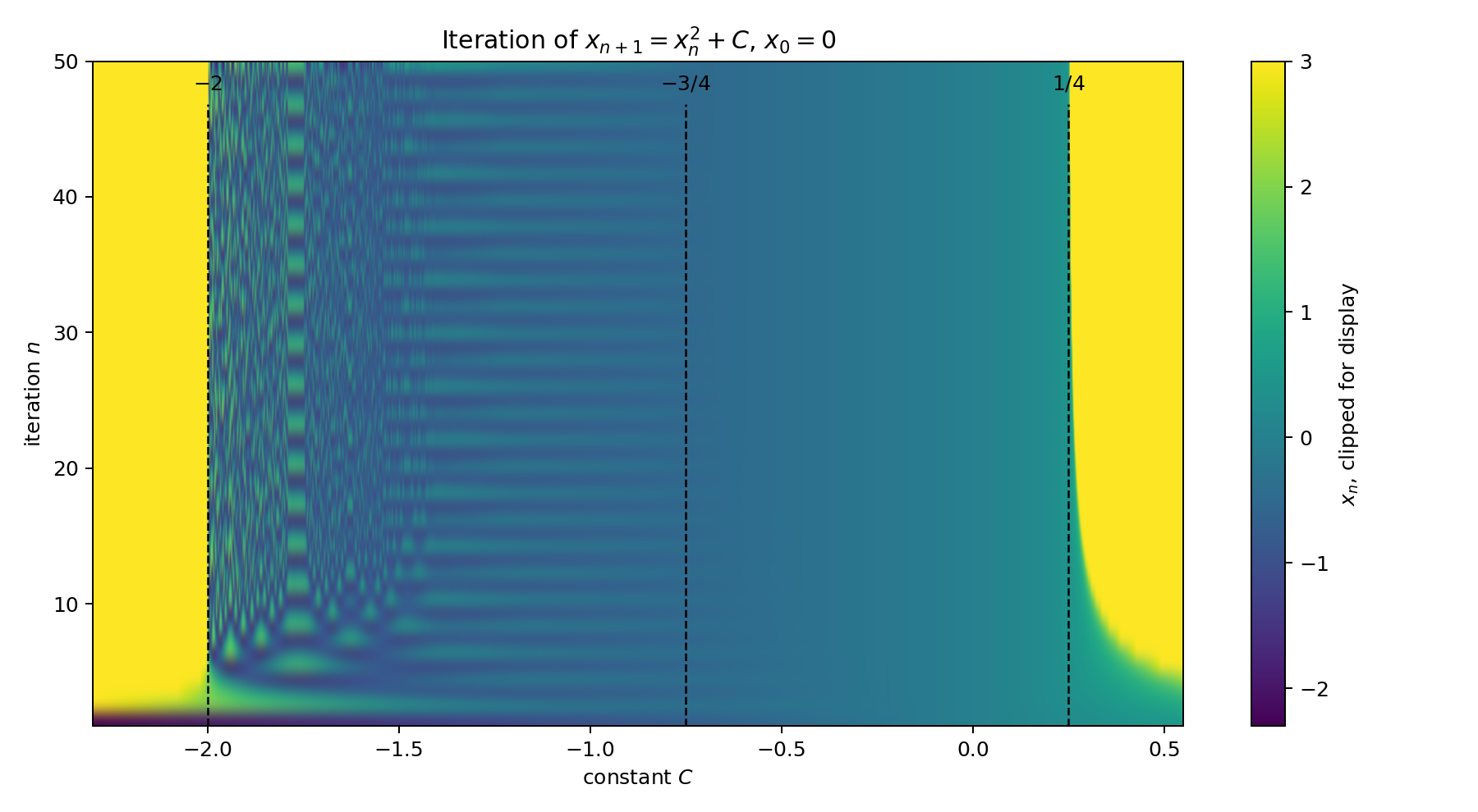
Instead of checking a few hand-picked values of $C$, we can scan a whole interval. In the next picture, the horizontal axis is the parameter $C$, the vertical axis is the iteration number $n$, and the color shows the value of $x_n$. The bright saturated regions are where the orbit has escaped so hard that the plot has to clip the value just to remain readable.

Iterating $x_{n+1}=x_n^2+C$ from $x_0=0$. The dashed lines mark $C=-2$, $C=-3/4$, and $C=1/4$. Outside $[-2,1/4]$, the orbit escapes. Between $-3/4$ and $1/4$, it settles to a fixed value. Between $-2$ and $-3/4$, it remains bounded but starts to split into oscillatory and chaotic behavior.

This picture is already suspiciously complicated on the left. The region $C < -2$ runs away, the region $C > 1/4$ runs away, but the strip between $-2$ and $-3/4$ is not boringly convergent. It contains bands, splits, and thin structure: the orbit is bounded, but it keeps oscillating between several stable values.

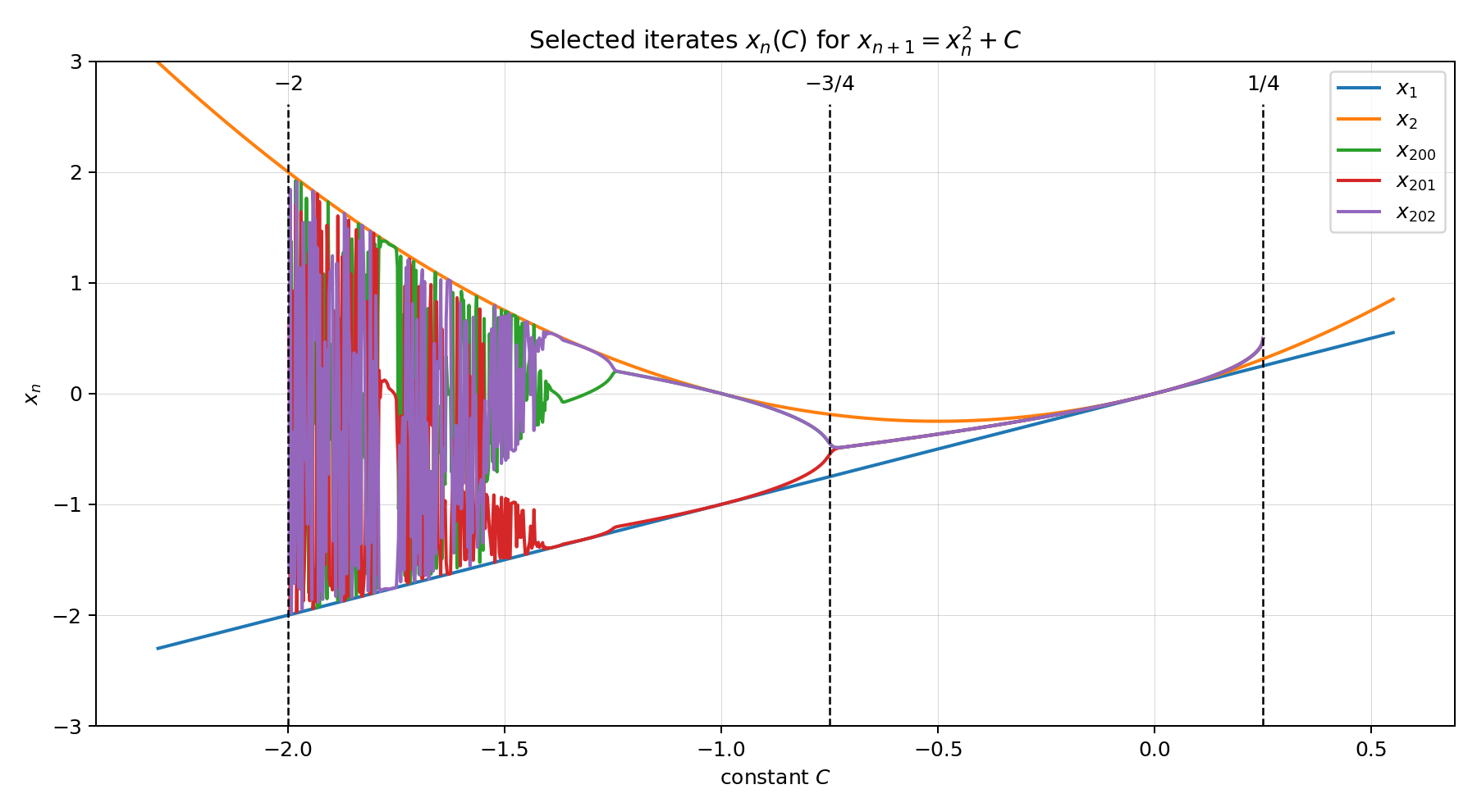
Another way to see the same transition is to plot $x_n$ as a function of $C$ for several different iteration numbers. Early iterates are smooth curves. Later iterates fold, split, and pile up. By the time we compare consecutive late iterates like $x_{200}$, $x_{201}$, and $x_{202}$, the convergent region has collapsed onto a single curve, while the oscillatory region has separated into different branches.

Selected functions $C \mapsto x_n(C)$. In the fixed-point region, late iterates lie almost on top of one another. In the bounded oscillatory region, consecutive late iterates separate into branches, exposing the period-doubling structure.

The table is only a handful of snapshots. The plots show the structure behind them. For real $C$, the orbit of $0$ stays bounded exactly on $[-2,1/4]$. The right-hand part, $[-3/4,1/4]$, is the tame region where the sequence settles to a fixed point. The left-hand part, $[-2,-3/4)$, is still bounded, but it is no longer tame: the orbit can cycle, double its period, and eventually wander chaotically.

AsideWhy these real intervals appear Show proof Hide proof

Let

$$ f_C(x) = x^2 + C, \qquad x_0 = 0, \qquad x_{n+1} = f_C(x_n). $$

A convergent orbit must approach a fixed point $L$, which must satisfy $L = f_C (L)$, so

$$ L = L^2 + C. $$

In other words, if the orbit lands exactly on $L$, it stays there forever.

We can rewrite this relation for $C$,

$$ C = L - L^2. $$

The convergence towards the fixed point can be examined by considering a value slightly off $L$:

$$ x_n = L + \varepsilon_n $$

where $\varepsilon_n$ is a tiny error from the fixed point $L$.

The next iterate is

$$ x_{n+1} = f_C (L + \varepsilon_n) $$

Which, for small $\varepsilon_n$ can be expanded into Taylor series in $\varepsilon_n$:

$$ x_{n+1} \approx f_C (L) + f^\prime_C (L) \varepsilon_n $$

However, since $L$ is a fixed point of $f_C$, then $f_C (L) = L$ and thus

$$ x_{n+1} \approx L + f^\prime_C (L) \varepsilon_n $$

Now, we assume that $x_{n+1}$ can also be written as $L$ with a small correction, $x_{n+1} = L + \varepsilon_{n+1}$. This leaves us with the following equation for the error propagation:

$$ \varepsilon_{n+1} \approx f^\prime_C (L) \varepsilon_n $$

For the convergence to happen, the fixed point needs to be attractive, i.e. $\lvert \varepsilon_{n+1} \rvert < \lvert \varepsilon_n \rvert$, which happens when

$$ \lvert f_C'(L) \rvert = \lvert 2L \rvert < 1, $$

with the endpoint cases $\lvert 2L \rvert=1$ giving the slower borderline behavior. Thus the attracting range is governed by

$$ -\frac{1}{2} \leq L \leq \frac{1}{2}. $$

On that interval, the function $C=L-L^2$ ranges from $-3/4$ to $1/4$. That gives the fixed-point convergence interval

$$ -\frac{3}{4} \leq C \leq \frac{1}{4}. $$

This explains the fixed-point convergence interval, but boundedness is slightly wider. The fixed-point argument already gives boundedness on $[-3/4,1/4]$, so it remains to check the left interval $[-2,-3/4]$.

Assume that $-2 \leq C \leq -3/4$. We will show, by induction, that for all $n\geq 1$,

$$ C \leq x_n \leq C^2+C. $$

The base case holds because

$$ x_1=C, \qquad x_2=C^2+C. $$

Now assume that

$$ C \leq x_n \leq C^2+C. $$

Then

$$ 0 \leq x_n^2 \leq \max\left(C^2,\,(C^2+C)^2\right). $$

But

$$ (C^2+C)^2 = C^4+2C^3+C^2 = C^2 + C^3(C+2). $$

For $-2\leq C\leq -3/4$, we have $C^3\leq 0$ and $C+2\geq 0$, so

$$ C^3(C+2)\leq 0. $$

Therefore

$$ (C^2+C)^2 \leq C^2, $$

and hence

$$ 0 \leq x_n^2 \leq C^2. $$

Adding $C$ everywhere gives

$$ C \leq x_n^2+C \leq C^2+C. $$

Since $x_{n+1}=x_n^2+C$, this is exactly

$$ C \leq x_{n+1} \leq C^2+C. $$

So the interval $[C,C^2+C]$ traps the orbit, and the orbit is bounded for every $C\in[-2,-3/4]$.

Outside $[-2,1/4]$, the orbit escapes. If $C>1/4$, then the equation $L=L^2+C$ has no real solution, so the orbit cannot settle to a real fixed point; starting from $0$, it eventually increases without bound. If $C<-2$, then $x_1=C<-2$ and $x_2=C^2+C>2$, after which the squaring term drives the orbit to larger and larger positive values.

So, for the real one-dimensional map:

$$ \text{bounded orbit from }0: \quad -2 \leq C \leq \frac{1}{4}, $$ $$ \text{fixed-point convergence:} \quad -\frac{3}{4} \leq C \leq \frac{1}{4}. $$

The interval $[-2,-3/4)$ is the fun warning sign: bounded does not necessarily mean convergent.

This result is intriguing, but it is still not very visual. A real number can only move left and right on a line. To get to the fun picture everyone is surely waiting on by now, we let both the starting value and the parameter live in the complex plane. The same little rule,

$$ z_{n+1} = z_n^2 + c, $$

now acts as a sorting machine on the complex plane: for which values of $c$ does the orbit of $z=0$ remain bounded, and for which does it escape? The boundary between those two outcomes is where the plain recurrence turns into the Mandelbrot set.

Since $z$ and $c$ are now complex numbers, we can represent them in the complex plane using their real and imaginary parts. Writing

$$ \begin{aligned} z_n &= a_n + i b_n \\ c &= x + i y \end{aligned} $$

we can rewrite the iteration equation for $z$ as follows

$$ \begin{aligned} a_{n+1} &= a_n^2 - b_n^2 + x \\ b_{n+1} &= 2 a_n b_n + y \end{aligned} $$

So every point $c=x+iy$ in the complex plane gives us a different orbit of the starting value $z_0=0$. To decide whether that orbit is escaping, we watch its modulus,

$$ \lvert z_n \rvert = \sqrt{a_n^2+b_n^2}. $$

For this map, once an iterate satisfies $\lvert z_n \rvert > 2$, the orbit is guaranteed to escape to infinity. If no iterate crosses that threshold after many steps, we treat the point as bounded for the purposes of the picture.

The fine structure of the boundary is not something we can simply draw from a closed-form formula. So we use a crude and naive approach: take a grid of points in the complex plane, treat each point as a candidate value of $c$, iterate the map from $z_0=0$, and check whether the orbit appears bounded or escapes. Then we color the point accordingly. Even this crude experiment is enough for the Mandelbrot set to begin revealing itself.

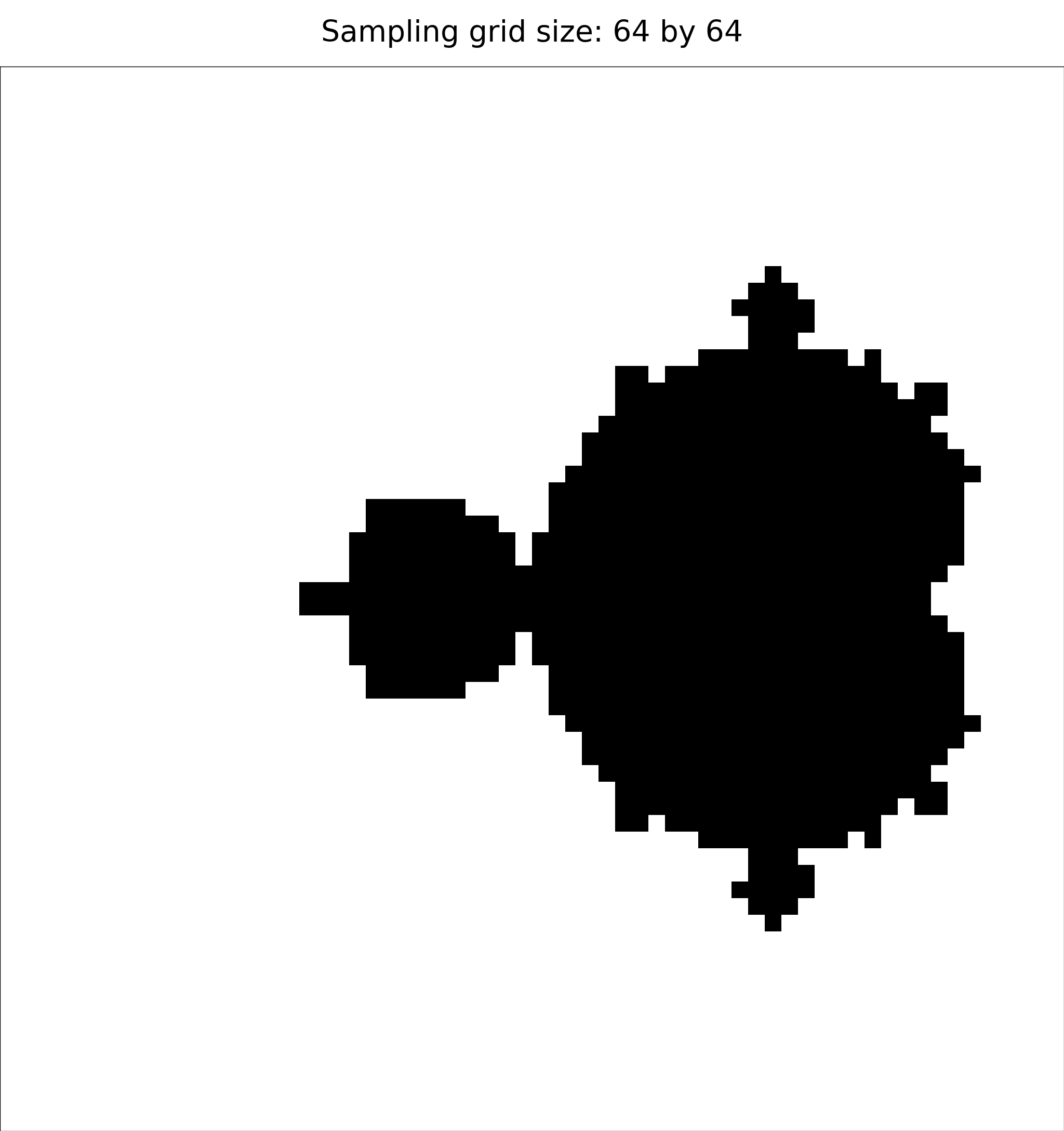
At first, we keep the experiment deliberately brutal: no colors or special treatment of the boundary. A point is black if its orbit survives the chosen number of iterations, and white if it escapes. This is not yet a proof of membership in the Mandelbrot set, because a point that survives many iterations could still escape later. But it is a perfectly good numerical first pass: the black region is our current approximation to the set.

The carousel below shows the same region of the complex plane sampled on finer and finer grids. The shape does not change; only our sampling of it improves. At low resolution, the set looks like a blocky silhouette. As the grid gets finer, the main cardioid, the large bulb on the left, the smaller satellite bulbs, and the rough boundary become much clearer.

Black/white escape test for the same region of the complex plane. Black points did not escape within the iteration limit; white points did. Current grid: 64 × 64.

The black-and-white version is useful because it shows the essential yes/no question: bounded or escaping? But it throws away a lot of information. Escaping points do not all behave the same way. Some fly away almost immediately, while others hover near the boundary for many iterations before finally leaving. Likewise, the bounded-looking interior is not uniform. Some regions settle to one attracting value, while others settle into repeating cycles.

So we can reuse the same computation, but color it more honestly. Outside the set, the color records escape speed: pale regions escape quickly and are dynamically far from the interesting boundary, while stronger colors mark points that escape slowly. Inside the set, the color records the detected attracting period after the orbit has settled: dark blue means fixed-point convergence, blue means period-2 oscillation, teal means period-3, green means period-4, yellow-green means period-5, orange means period-6, red means period-7, and purple means period-8. Black interior points are bounded in this numerical test, but were not classified into one of those periods; they may be higher-period, boundary-adjacent, or simply unresolved at this iteration depth.

Colored escape-time and interior-period view of the same grid experiment. Outside colors show escape speed; inside colors show the detected attracting period. Current grid: 64 × 64.

In the colored version we can see that the points far away from the set escape quickly and fade toward the background. Points near the boundary escape slowly, which is why the exterior develops colored halos and filaments. Inside, the large regions of stable behavior are the complex-plane relatives of what we already saw on the real line: convergence, oscillation, period-doubling, and more complicated bounded behavior.

It is not an accident that the interior segments of our Mandelbrot set feature unique periodic behavior per segment. The interior of the Mandelbrot set contains infinitely many bulb-like regions, called hyperbolic components, each organized around an attracting periodic cycle. For example, the main cardioid (bulb-looking thing) is a 1-period component, meaning the iterations $z \to z^2 + c$ settle to a single value (depending on $c$) within the interior of the cardioid. Such limiting value can then be obtained by solving

$$ z = z^2 + c $$

for $z$.

AsideSingle-valued cardioid Show Hide

Let’s assume, that the iteration $z \to z^2 + c$ has an attracting fixed point $z$. In that case, the value can be obtained by solving

$$ z = z^2 + c $$

Moreover, similar to the real case, once the orbit is close to this fixed point, small errors shrink if

$$ \lvert f^\prime_c(z) \rvert = \lvert 2z \rvert < 1 $$

The region of values $z$ that satisfy $2 \lvert z \rvert < 1$ can be parameterized as

$$ z = \frac{r}{2} e^{i \phi}, \qquad \begin{aligned} r &\in [0, 1) \\ \phi &\in [0, 2 \pi) \end{aligned} $$

In that case, we have:

$$ c = z - z^2 = \frac{r}{2} e^{i \phi} - \frac{r^2}{4} e^{2 i \phi} $$

The boundary of this region can be obtained by setting $r = 1$, which results in the famous cardioid shape.

The single value for each $c$ can be obtained by solving the quadratic equation for $z$

$$ z = \frac{1}{2} \left( 1 \pm \sqrt{1 - 4 c} \right) $$

To pick the correct branch we recall, that the actual attracting limit satisfies $2 \lvert z \rvert < 1$. Here we see, that for $c = 0$ only the negative branch satisfies $2 \lvert z \rvert < 1$. To prove that the correct branch is

$$ z = \frac{1}{2} \left( 1 - \sqrt{1 - 4 c} \right) $$

throughout the entire interior of the cardioid, we look at the relationship between the two roots. If one root is $z$, the other root must be $1 - z$, because the two roots of $z^2 - z + c = 0$ sum to 1. Therefore, if one root satisfies $\lvert z \rvert < 1/2$, the other, by the reverse triangle inequality, satisfies

$$ \lvert 1 - z \rvert \geq \lvert 1 - \lvert z \rvert \rvert = 1 - \lvert z \rvert > 1/2 $$

So at most one fixed point can be attracting. Since the negative branch gives $z = 0$ at $c = 0$, it is the attracting branch throughout the interior of the cardioid.

The two roots could only meet if

$$ z_+ = z_- \quad \implies \quad \sqrt{1 - 4 c} = 0 $$

which gives $c = 1/4$, the cusp of the cardioid. This point lies on the boundary, not inside the region.

To sum up, we have shown, that the region where the map has an attracting fixed point is described parameterically as

$$ c = \frac{r}{2} e^{i \phi} - \frac{r^2}{4} e^{2 i \phi}, \qquad \begin{aligned} r &\in [0, 1) \\ \phi &\in [0, 2 \pi) \end{aligned} $$

And the value it converges to is

$$ z = \frac{1}{2} \left( 1 - \sqrt{1 - 4 c} \right) $$

This is the main cardioid of the Mandelbrot set.

Within the disk located to the left of the main cardioid, the iterations eventually settle into two repeating values:

$$ z_1 (c) \to z_2 (c) \to z_1 (c) \to \cdots $$

In this case, the limiting values can be obtained by solving

$$ z = (z^2 + c)^2 + c, $$

i.e. nesting the iteration twice.

AsideDouble-valued circle Show Hide

Let’s now assume, that the iteration $z \to z^2 + c$ leads to two alternating values,

$$ z_1 (c) \to z_2 (c) \to z_1 (c) \to \cdots $$

In that case, we have to obtain back the same value $z$ after nesting the iteration twice:

$$ z = f_c(f_c(z)) = (z^2 + c)^2 + c $$

However, care must be taken when analyzing this equation. In addition to true 2-periodic behavior, this equation also contains the single-valued case, as certainly if $z = z^2 + c$ then also $z = (z^2 + c)^2 + c$ (the inverse is not true). We can easily get rid of the trivial, single-valued case by factoring out $z^2 - z + c$ from the polynomial. This can be done with a simple guess:

$$ z^4 + 2 c z^2 - z + c^2 + c = (z^2 - z + c) (z^2 + z + c + 1) $$

We know, that the first part, $z^2 - z + c$ hides the single-valued cardioid, so the 2-period region must be described by

$$ z^2 + z + c + 1 = 0. $$

The two roots of this equation are the two values of the alternating cycle. Let us call them $z_1$ and $z_2$. By Vieta’s formulas applied to

$$ z^2 + z + c + 1 = 0, $$

we have

$$ z_1 + z_2 = -1, \qquad z_1 z_2 = c + 1. $$

Also, from the same equation,

$$ z^2 + c = -z - 1. $$

Since $f_c(z) = z^2 + c$, this means

$$ f_c(z) = -z - 1. $$

So if one point of the cycle is $z_1$, the other one is

$$ z_2 = -z_1 - 1, $$

and applying the map again returns us to $z_1$.

Now we need to ask when this two-cycle is attracting. Since one full cycle takes two iterations, the relevant multiplier is

$$ \lambda = f_c'(z_1) f_c'(z_2). $$

Because $f_c’(z) = 2z$, we get

$$ \lambda = (2z_1)(2z_2) = 4 z_1 z_2. $$

Using $z_1 z_2 = c + 1$, this becomes

$$ \lambda = 4(c+1). $$

The two-cycle is attracting when small errors shrink after a full cycle, so

$$ |\lambda| < 1. $$

Therefore,

$$ |4(c+1)| < 1, $$

or equivalently

$$ |c+1| < \frac{1}{4}. $$

This is exactly a circle centered at $c=-1$ with radius $1/4$. Thus the double-valued component can be parametrized as

$$ c = -1 + \frac{r}{4}e^{i\phi}, \qquad r \in [0,1), \qquad \phi \in [0,2\pi). $$

The boundary is obtained by setting $r=1$.

Generally, $n$-periodic regions can be explored by considering the $n$-fold nesting

$$ z = f_c(f_c(f_c(\cdots))) \equiv f_c^n (z) $$

At this point the algebra starts sticking out its nasty beak and talons. For period 1, the equations collapse into the cardioid. For period 2, they collapse into a circle. For period 3 and above, the same idea still works, but the expanded polynomials quickly become too unpleasant to write by hand.

So instead of trying to draw these components by sampling a dense grid of pixels, we can build them more directly.

Each attracting period-$n$ component has a special center. At that center, the critical point $0$ lies exactly on the cycle:

$$ f_c^n(0)=0. $$

This gives us the centers of the components.

Then, to fill the component, we use the multiplier of the attracting cycle,

$$ \lambda = (f_c^n)'(z). $$

For $f_c(z)=z^2+c$, this is

$$ \lambda = (2z_0)(2z_1)\cdots(2z_{n-1}). $$

The component interior corresponds to

$$ |\lambda|<1. $$

So instead of sampling the Mandelbrot plane directly, we sample a clean disk

$$ \lambda = r e^{i\phi}, \qquad 0\leq r<1, $$

and numerically solve for the corresponding value of $c$.

This gives a clean polygon mesh for each component. For every sampled $c$, the attracting cycle gives $n$ values

$$ z_0,\ z_1,\ \dots,\ z_{n-1}. $$

Those become the $n$ sheets in the final visualization. The height is $\lvert z_j\rvert$, and the color is the phase $\arg(z_j)$.

AsideHow the component atlas is generated Show method Hide method

The numerical construction has two stages.

First, we find the centers. Define

$$ P_n(c)=f_c^n(0). $$

The roots of $P_n(c)$ contain centers whose exact periods divide $n$. To keep only exact period $n$, we divide out the lower-period center polynomials:

$$ \Psi_n(c) = \frac{P_n(c)} {\prod_{d\mid n,\ d<n}\Psi_d(c)}. $$

For example,

$$ \Psi_3(c)=c^3+2c^2+c+1, $$

whose three roots are the centers of the three period-3 components.

Second, for each center $c_i$, we fill the component using multiplier coordinates. For a chosen multiplier

$$ \lambda = r e^{i\phi}, \qquad r<1, $$

we solve the two equations

$$ f_c^n(z)=z, $$ $$ (f_c^n)'(z)=\lambda. $$

At the center, the starting solution is especially simple:

$$ \lambda=0,\qquad c=c_i,\qquad z=0. $$

Then we move outward in small steps in $\lambda$-space, using each previous solution as the starting guess for the next one. This avoids trying to recover the component shape from a dense pixel grid.

Once one point $z_0$ of the attracting cycle is found, the rest are obtained for free:

$$ z_1=z_0^2+c,\qquad z_2=z_1^2+c,\qquad \dots $$

For a period-$n$ component, this gives $n$ sheets. Each sheet is plotted over the same component in the $c$-plane, with height $\lvert z_j\rvert$ and color $\arg(z_j)$.

The final experiment below shows an atlas of the stable interior pieces: the attracting periodic components. Each component is sampled in its own multiplier coordinate, then lifted into 3D.

The base of each colored sheet lives in the familiar $c$-plane. The height is $\lvert z_j\rvert$, where $z_j$ is one point of the attracting cycle. The color records the phase $\arg(z_j)$. So a period-$n$ component does not become one surface, but $n$ related sheets stacked over the same region. The thin vertical guide lines mark component centers, where the critical point $0$ lies exactly on the periodic cycle.

Interactive demo Mandelbrot component atlas Large interactive WebGL visualization. The preview is static; the full atlas loads only after clicking.

Static preview; the interactive WebGL version loads only after clicking.

Loading atlas… This can take a few seconds.

Open full screen

Drag to rotate, scroll or pinch to zoom. On phones, opening the atlas full screen may work better than using it inside the page.

While this render does not show the full Mandelbrot story (such as exotic behavior at the boundary), it builds a stable skeleton: the places where the iteration settles into attracting cycles, unfolded into branching colored sheets.