So let’s begin with the least glamorous toy model possible. Pick a number $C$, start at $x_0 = 0$, and repeat

That is the whole machine. No geometry yet, no colors, no complex numbers, no pretty fractal boundary. Just one real number being fed back into the same rule over and over again. But already, something interesting happens: for some values of $C$, the sequence calmly settles down; for others it stays bounded but refuses to settle into one value; and beyond a certain range it runs away to infinity.

A few sample values make the split visible:

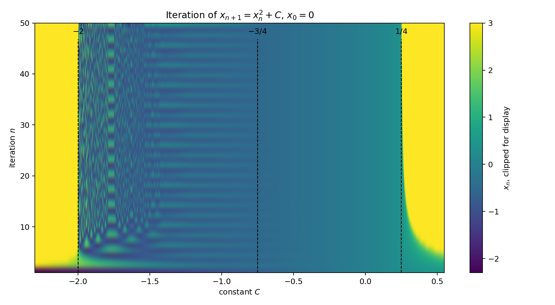
Instead of checking a few hand-picked values of $C$, we can scan a whole interval. In the next picture, the horizontal axis is the parameter $C$, the vertical axis is the iteration number $n$, and the color shows the value of $x_n$. The bright saturated regions are where the orbit has escaped so hard that the plot has to clip the value just to remain readable.

This picture is already suspiciously complicated on the left. The region $C < -2$ runs away, the region $C > 1/4$ runs away, but the strip between $-2$ and $-3/4$ is not boringly convergent. It contains bands, splits, and thin structure: the orbit is bounded, but it keeps oscillating between several stable values.

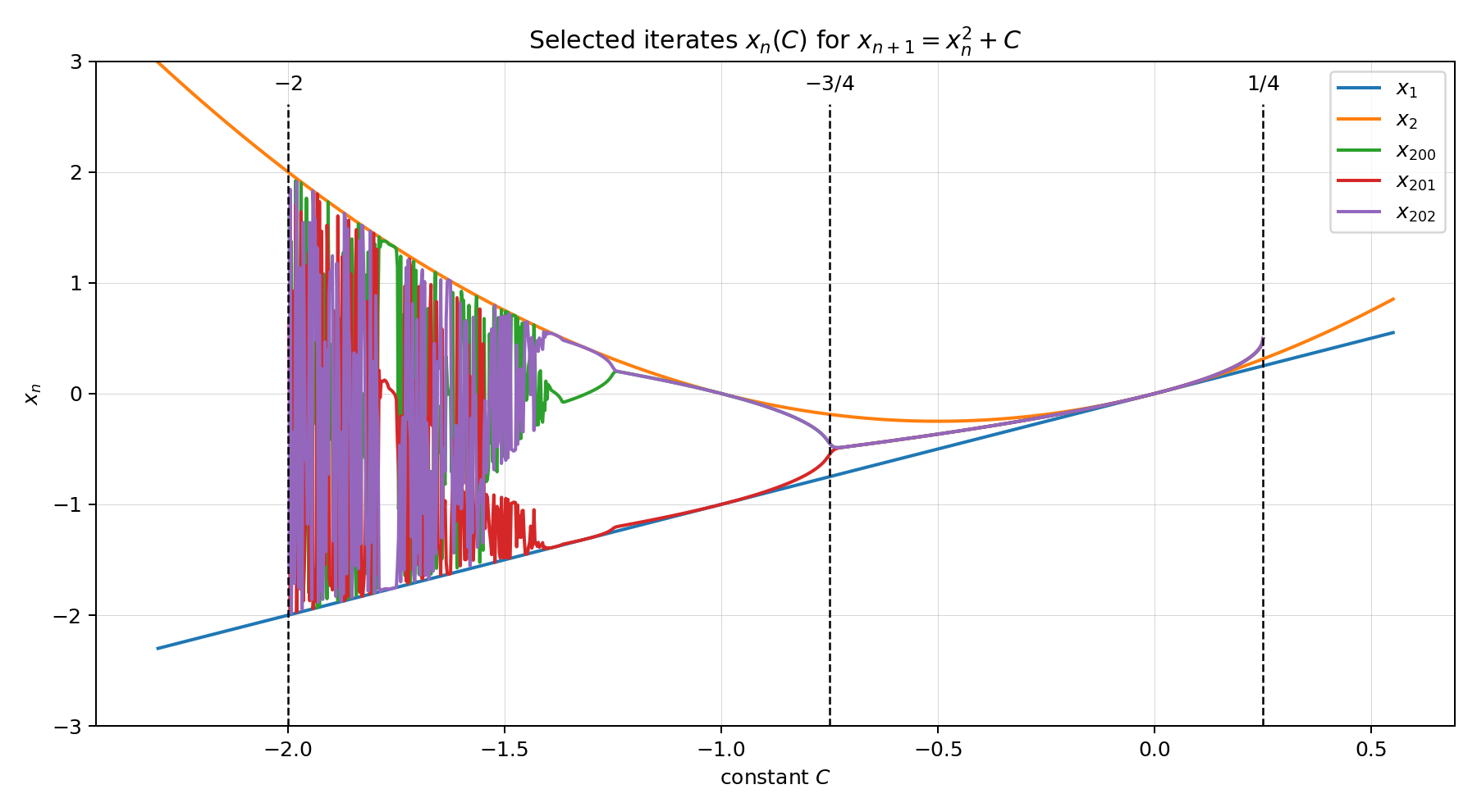
Another way to see the same transition is to plot $x_n$ as a function of $C$ for several different iteration numbers. Early iterates are smooth curves. Later iterates fold, split, and pile up. By the time we compare consecutive late iterates like $x_{200}$, $x_{201}$, and $x_{202}$, the convergent region has collapsed onto a single curve, while the oscillatory region has separated into different branches.

The table is only a handful of snapshots. The plots show the structure behind them. For real $C$, the orbit of $0$ stays bounded exactly on $[-2,1/4]$. The right-hand part, $[-3/4,1/4]$, is the tame region where the sequence settles to a fixed point. The left-hand part, $[-2,-3/4)$, is still bounded, but it is no longer tame: the orbit can cycle, double its period, and eventually wander chaotically.

This result is intriguing, but it is still not very visual. A real number can only move left and right on a line. To get to the fun picture everyone is surely waiting on by now, we let both the starting value and the parameter live in the complex plane. The same little rule,

now acts as a sorting machine on the complex plane: for which values of $c$ does the orbit of $z=0$ remain bounded, and for which does it escape? The boundary between those two outcomes is where the plain recurrence turns into the Mandelbrot set.

Since $z$ and $c$ are now complex numbers, we can represent them in the complex plane using their real and imaginary parts. Writing

we can rewrite the iteration equation for $z$ as follows

So every point $c=x+iy$ in the complex plane gives us a different orbit of the starting value $z_0=0$. To decide whether that orbit is escaping, we watch its modulus,

For this map, once an iterate satisfies $\lvert z_n \rvert > 2$, the orbit is guaranteed to escape to infinity. If no iterate crosses that threshold after many steps, we treat the point as bounded for the purposes of the picture.

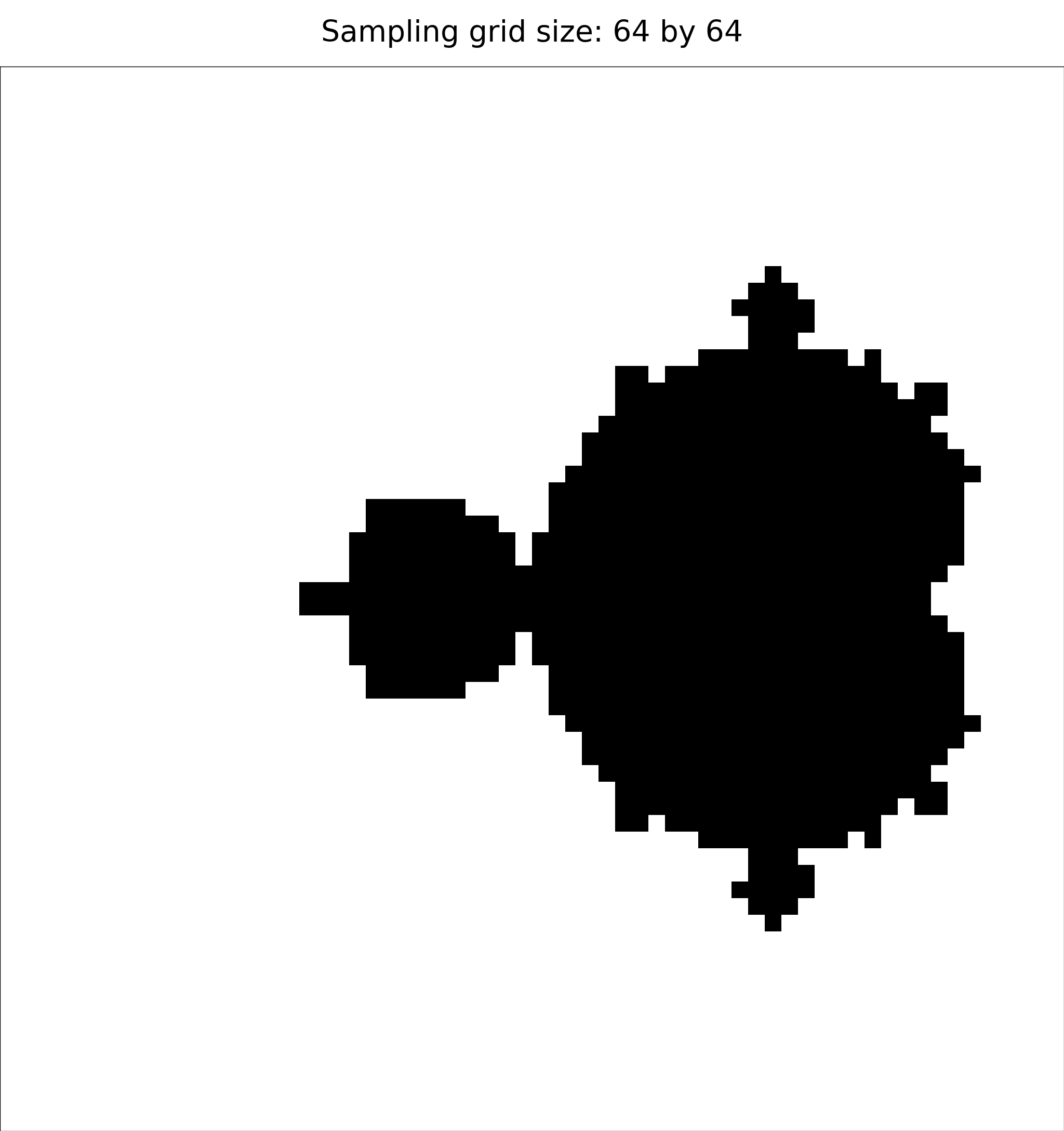
The fine structure of the boundary is not something we can simply draw from a closed-form formula. So we use a crude and naive approach: take a grid of points in the complex plane, treat each point as a candidate value of $c$, iterate the map from $z_0=0$, and check whether the orbit appears bounded or escapes. Then we color the point accordingly. Even this crude experiment is enough for the Mandelbrot set to begin revealing itself.

At first, we keep the experiment deliberately brutal: no colors or special treatment of the boundary. A point is black if its orbit survives the chosen number of iterations, and white if it escapes. This is not yet a proof of membership in the Mandelbrot set, because a point that survives many iterations could still escape later. But it is a perfectly good numerical first pass: the black region is our current approximation to the set.

The carousel below shows the same region of the complex plane sampled on finer and finer grids. The shape does not change; only our sampling of it improves. At low resolution, the set looks like a blocky silhouette. As the grid gets finer, the main cardioid, the large bulb on the left, the smaller satellite bulbs, and the rough boundary become much clearer.

← →

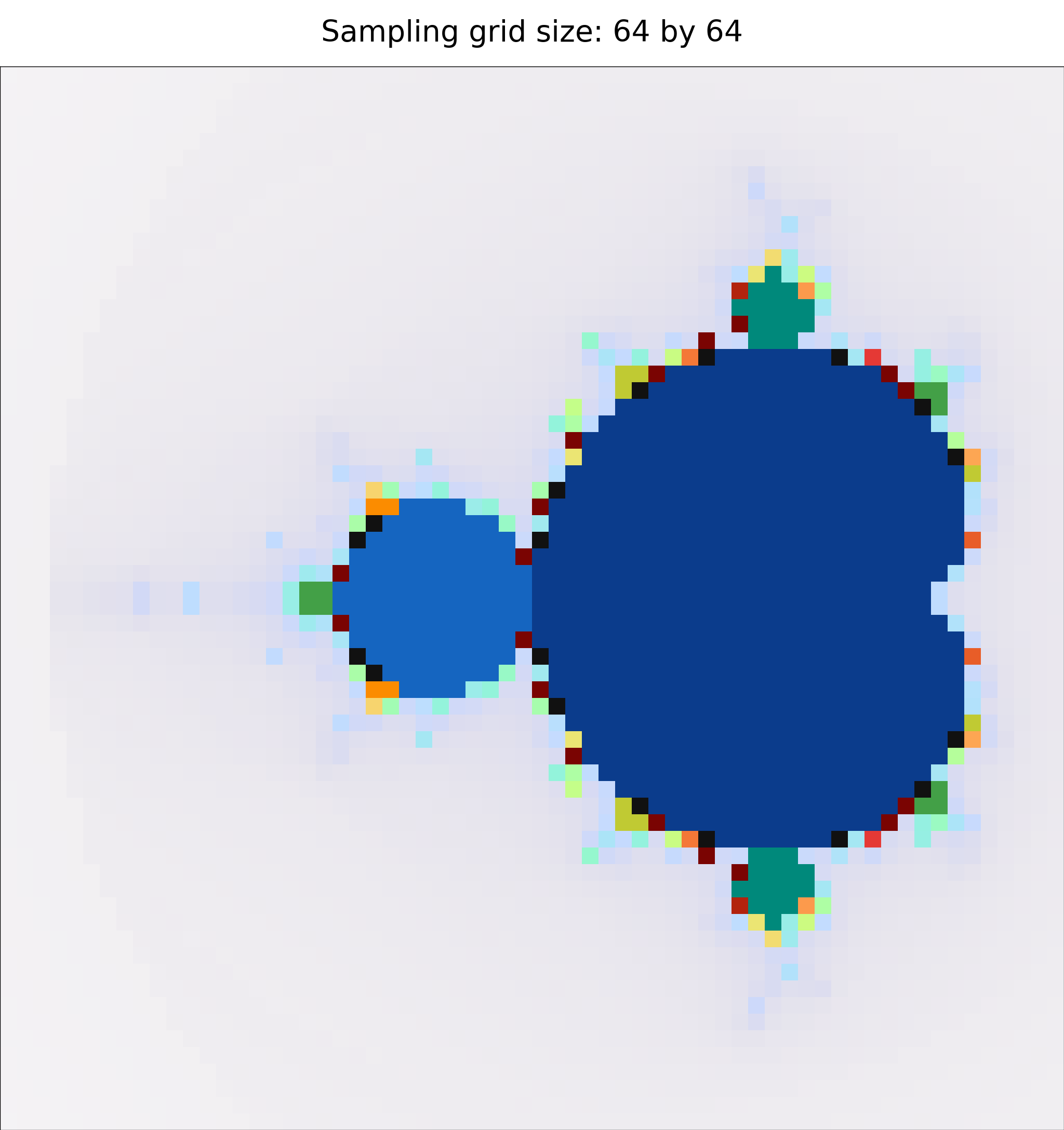
The black-and-white version is useful because it shows the essential yes/no question: bounded or escaping? But it throws away a lot of information. Escaping points do not all behave the same way. Some fly away almost immediately, while others hover near the boundary for many iterations before finally leaving. Likewise, the bounded-looking interior is not uniform. Some regions settle to one attracting value, while others settle into repeating cycles.

So we can reuse the same computation, but color it more honestly. Outside the set, the color records escape speed: pale regions escape quickly and are dynamically far from the interesting boundary, while stronger colors mark points that escape slowly. Inside the set, the color records the detected attracting period after the orbit has settled: dark blue means fixed-point convergence, blue means period-2 oscillation, teal means period-3, green means period-4, yellow-green means period-5, orange means period-6, red means period-7, and purple means period-8. Black interior points are bounded in this numerical test, but were not classified into one of those periods; they may be higher-period, boundary-adjacent, or simply unresolved at this iteration depth.

← →

In the colored version we can see that the points far away from the set escape quickly and fade toward the background. Points near the boundary escape slowly, which is why the exterior develops colored halos and filaments. Inside, the large regions of stable behavior are the complex-plane relatives of what we already saw on the real line: convergence, oscillation, period-doubling, and more complicated bounded behavior.

It is not an accident that the interior segments of our Mandelbrot set feature unique periodic behavior per segment. The interior of the Mandelbrot set contains infinitely many bulb-like regions, called hyperbolic components, each organized around an attracting periodic cycle. For example, the main cardioid (bulb-looking thing) is a 1-period component, meaning the iterations $z \to z^2 + c$ settle to a single value (depending on $c$) within the interior of the cardioid. Such limiting value can then be obtained by solving

for $z$.

Within the disk located to the left of the main cardioid, the iterations eventually settle into two repeating values:

In this case, the limiting values can be obtained by solving

i.e. nesting the iteration twice.

Generally, $n$-periodic regions can be explored by considering the $n$-fold nesting

At this point the algebra starts sticking out its nasty beak and talons. For period 1, the equations collapse into the cardioid. For period 2, they collapse into a circle. For period 3 and above, the same idea still works, but the expanded polynomials quickly become too unpleasant to write by hand.

So instead of trying to draw these components by sampling a dense grid of pixels, we can build them more directly.

Each attracting period-$n$ component has a special center. At that center, the critical point $0$ lies exactly on the cycle:

This gives us the centers of the components.

Then, to fill the component, we use the multiplier of the attracting cycle,

For $f_c(z)=z^2+c$, this is

The component interior corresponds to

So instead of sampling the Mandelbrot plane directly, we sample a clean disk

and numerically solve for the corresponding value of $c$.

This gives a clean polygon mesh for each component. For every sampled $c$, the attracting cycle gives $n$ values

Those become the $n$ sheets in the final visualization. The height is $\lvert z_j\rvert$, and the color is the phase $\arg(z_j)$.

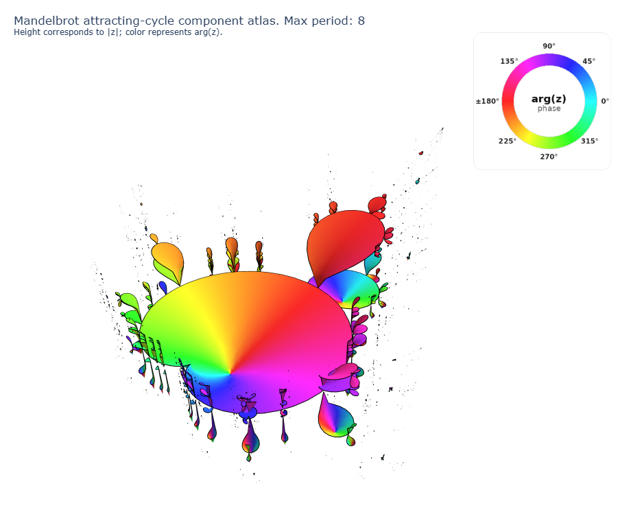
The final experiment below shows an atlas of the stable interior pieces: the attracting periodic components. Each component is sampled in its own multiplier coordinate, then lifted into 3D.

The base of each colored sheet lives in the familiar $c$-plane. The height is $\lvert z_j\rvert$, where $z_j$ is one point of the attracting cycle. The color records the phase $\arg(z_j)$. So a period-$n$ component does not become one surface, but $n$ related sheets stacked over the same region. The thin vertical guide lines mark component centers, where the critical point $0$ lies exactly on the periodic cycle.

Interactive demo Mandelbrot component atlas Large interactive WebGL visualization. The preview is static; the full atlas loads only after clicking.

Load demo Static preview; the interactive WebGL version loads only after clicking.

Loading atlas… This can take a few seconds.

Open full screen

While this render does not show the full Mandelbrot story (such as exotic behavior at the boundary), it builds a stable skeleton: the places where the iteration settles into attracting cycles, unfolded into branching colored sheets.

What started as a fairly plain GitHub Pages site has now been reorganized into something cleaner, nicer to use, and much easier to maintain. The goal was to turn it into something more intentional and maintainable: better spacing, nicer typography, cleaner cards, reusable layouts, and a more coherent structure across the whole site.

The biggest visible change is the new design. The homepage now has a clearer introduction, section cards for research, BeamNG projects, and writing, plus a cleaner preview of recent posts. Project and post cards now behave consistently: the whole card is clickable, the hover effect is shared, and only the title is highlighted instead of the entire text turning into one giant link.

Under the hood, the site is now much more modular. Repeated pieces of layout have been moved into reusable Jekyll includes, so I do not have to copy the same chunks of HTML everywhere. Project pages, galleries, stats boxes, figures, post lists, and cards can now be controlled from a smaller number of shared components. This should make future changes much less painful.

The BeamNG section also got reorganized into proper project-style pages. Instead of each page being a pile of custom markup, the structure is now more predictable: metadata lives in front matter, content lives in Markdown, and reusable includes handle the repeated visual pieces.

There were also a few quality-of-life fixes: cleaner local development with live reload, better handling of custom post summaries, improved card previews, less fragile styling, and a clearer separation between website content and local-only files like notebooks, raw data, and generated assets.

This is still a personal site, so it will keep evolving. But now it finally feels like a better foundation; flexible enough to grow, and just polished enough that I am no longer embarrassed to put it on a proper domain.

See Why Gaussian? Part I: tossing dice for part 1!

See Why Gaussian? Part II: continuous additive processes for part 2!

In the first part of this series, we saw how a discrete random variable (like a roll of a die), when accumulated across independent trials, converges toward a Gaussian distribution. In the second part, we extended this to continuous variables - showing how, under mild conditions on their moments, the same convergence occurs.

In this post, we take a different path. Not all natural processes are additive. Some involve multiplication, cyclic variables, or nonlinear transformations. Yet, remarkably, the Gaussian often still emerges-sometimes not in the variable itself, but in a transformed version like its logarithm or phase. Let's explore these less-obvious routes to Gaussian behavior.

Multiplicative random processes

While the central limit theorem is traditionally associated with additive processes, many real-world systems operate multiplicatively. Fortunately, multiplication becomes addition in logarithmic space, so a wide array of CLT-like results still apply, just one transformation away. In fact, many systems that produce log-normal statistics are fundamentally multiplicative at their core.

Consider a few well-known examples: compound interest in finance, population growth with random fluctuations, or the cascade of returns in stock markets - all evolve by repeated multiplication of random factors. In such cases, taking the logarithm converts the product into a sum, and the central limit theorem applies to the log-transformed variable. As a result, the original variable becomes log-normally distributed.

One particularly elegant example comes from astrophysical fluid dynamics: the density structure in isothermal, supersonic turbulence. In such flows, density fluctuations are largely governed by shock waves. Each shock compresses the local density by a factor determined by the velocity field, so the density doesn't evolve additively, but multiplicatively. For isothermal shocks (where the adiabatic index $\gamma = 1$), the Rankine–Hugoniot jump condition simplifies to a density jump $\rho_2 / \rho_1 = m^2$, where (dimensionless) $m$ is the upstream Mach number; the speed of the shock reduced by the speed of sound. As gas elements traverse a sequence of shocks, the resulting density is repeatedly multiplied by factors drawn from the local velocity dispersion. To be clear, if a parcel of gas is affected by $n$ shocks passing through it, each propagating with some random local Mach number $m$, the resulting density will be

$$ \rho = \rho_0 \, m_1 \, m_2 \cdots m_n $$

Naturally, to understand the distribution of final densities, we must know how the local Mach number itself is distributed. In a turbulent flow, these are not fixed, but fluctuate based on the local velocity field. The precise form of the Mach number distribution depends on the turbulence driving and thermodynamic conditions, but it's generally broad and continuous, with most values clustered near the mean turbulent Mach number.

If we assume the Mach numbers $m_i$ for each shock are drawn independently from such a distribution (or more realistically, weakly correlated), then the logarithm of the final density becomes a sum of random terms:

$$ \log (\rho / \rho_0) + \log m_1 + \log m_2 + \cdots + \log m_n. $$

This is precisely the setup where the central limit theorem applies. Under fairly weak assumptions about the shape and variance of the $\log m$ distribution, the sum converges toward a Gaussian. Therefore, the logarithm of density, $s \equiv \log (\rho / \rho_0)$ follows a normal distribution, and the density itself follows a lognormal distribution:

But what does the distribution of local Mach numbers actually look like in a turbulent flow? Since the Mach number $m = v / c_s$ is just the velocity normalized by the sound speed, this really comes down to the statistics of local velocity magnitudes.

In an isothermal turbulent medium with no large-scale bulk motion, the three Cartesian components of velocity can be reasonably modeled as independent random variables drawn from a Gaussian distribution centered at zero-thanks to the central limit effect of countless random driving forces. When this is the case, the magnitude of the velocity (and hence the local Mach number) follows a Maxwell–Boltzmann distribution.

In three dimensions, the Maxwellian PDF for the Mach number $m$ takes the form:

$$ f (m) = \frac{4 \pi m^2}{(2 \pi \sigma^2)^{3/2}} \exp \left( - \frac{m^2}{2 \sigma^2} \right) $$

where $\sigma$ is the standard deviation of the underlying 1D velocity components (in units of the sound speed). This shape arises naturally when you compute the distribution of the magnitude of a 3D Gaussian vector. Most of the probability mass lies around the typical turbulent Mach number, but there's a non-negligible tail at high $m$, allowing for occasional strong shocks.

There's one important complication we need to address before we go further: real shock waves only occur when the flow is supersonic, that is, when the Mach number $m > 1$. If the flow is subsonic, information travels fast enough upstream to smooth out any discontinuity before a shock can form. In our setup, however, we're drawing Mach numbers from a continuous distribution (like the Maxwellian), which includes both subsonic and supersonic values.

So what happens to those subsonic samples in our model? Strictly speaking, they shouldn't correspond to shocks at all. But in turbulent flows, not every compressive or expansive feature is a perfect shock. There are also rarefaction waves, which are smooth expansions rather than discontinuous jumps. Unlike shocks, which compress the gas and increase the density, rarefactions decrease the density across a smooth gradient.

In our simplified picture, we can treat these rarefactions as "anti-shocks"; they still change the density by a multiplicative factor, but one that's less than one. A convenient way to model both compression and expansion statistically is to let each event (shock or rarefaction) multiply the density by a factor of $m^2$, even when $m < 1$. This may not match every microscopic detail, but it captures the essential multiplicative character of density evolution in turbulent media.

This Maxwellian form gives us a physically motivated, continuous distribution from which to draw the multiplicative shock factors $m^2$. With that foundation in place, we're finally ready to run a small numerical experiment.

Shocks as a random multiplicative process: numerical experiment

We'll simulate a parcel of gas undergoing a series of random isothermal shocks. Each shock multiplies the current density by $m^2$, where the Mach number $m$ is drawn from the Maxwellian distribution with some pre-defined $\sigma$. After a few such multiplicative steps, we'll examine the distribution of the resulting density.

Here's a Python code that will give us some distributions:

import numpy as np
import matplotlib.pyplot as plt
from scipy.stats import maxwell, norm, lognorm
from tqdm import tqdm
import os

import numpy as np
import matplotlib.pyplot as plt
from scipy.stats import maxwell, norm, lognorm
import os

def multiplicative_clt_demo(
    n=5,
    N=10000,
    bins=100,
    base_dir="",
    title="Multiplicative CLT Demo",
    filename="lognormal_plot.png",
    sigma=2.0,
    toggle_gaussian=True,
    toggle_lognormal=True,
    threshold=0.005
):
    # sample mach numbers from maxwellian
    log_density = np.zeros(N)
    for _ in tqdm(range(n), desc="Applying shocks", ascii=True):
        mach = maxwell.rvs(scale=sigma, size=N)
        log_density += 2 * np.log(mach)  # because shock_factors = mach^2

    # normalize the ensemble towards zero mean and unit variance
    mu = np.mean(log_density)
    std = np.std(log_density)
    log_density_norm = (log_density - mu) / std

    # we also need density for plotting
    density = np.exp(log_density_norm)
    mu = 0
    std = 1

    # --- LOG-DENSITY PLOT ---
    plt.figure(figsize=(8, 5))
    counts, bin_edges = np.histogram(log_density_norm, bins=bins, density=True)
    bin_width = bin_edges[1] - bin_edges[0]
    bin_centers = bin_edges[:-1]

    plt.bar(
        bin_centers, counts, width=bin_width,
        color="skyblue", edgecolor="none",
        align="edge", label="Normalized log-density")
    for x, height in zip(bin_centers, counts):
        plt.plot([x, x + bin_width], [height, height],
        color="black", linewidth=0.5)

    if toggle_gaussian:
        significant = counts > threshold * np.max(counts)
        x_min = bin_edges[np.argmax(significant)]
        x_max = bin_edges[::-1][np.argmax(significant[::-1])]
        x_range = x_max - x_min
        x = np.linspace(x_min - 0.1 * x_range, x_max + 0.1 * x_range, 1000)
        y = norm.pdf(x, loc=0, scale=1)
        plt.plot(x, y, 'k--', label="Ideal Normal Distribution")

    plt.title(f"{title}\nLog-density (n={n}, N={N}, σ={sigma})")
    plt.xlabel("Normalized log-density")
    plt.ylabel("Probability Density")
    plt.grid(True)
    plt.legend(loc="upper right")
    plt.ylim(top=max(counts.max(), y.max() if toggle_gaussian else 0) * 1.2)
    plt.xlim(x[0], x[-1])

    path_log = os.path.join(base_dir, "log_" + filename)
    plt.savefig(path_log, dpi=150)
    plt.close()
    print(f"Saved log-density plot to {path_log}")

    # --- DENSITY PLOT ---
    plt.figure(figsize=(8, 5))

    # Fix histogram x-axis range
    density_min = 0
    density_max = 10  # adjust as needed

    # Manually define bin edges and bin centers
    bin_edges_d = np.linspace(density_min, density_max, bins + 1)
    bin_width_d = bin_edges_d[1] - bin_edges_d[0]
    bin_centers_d = bin_edges_d[:-1]

    # Clip data to range
    density_clipped = density[
        (density >= density_min) &
        (density <= density_max)]
    counts_d, _ = np.histogram(density_clipped,
        bins=bin_edges_d, density=True)

    # Plot bars
    plt.bar(
        bin_centers_d,
        counts_d,
        width=bin_width_d,
        color="lightcoral",
        edgecolor="none",
        align="edge",
        label="Density"
    )

    for x, height in zip(bin_centers_d, counts_d):
        plt.plot([x, x + bin_width_d], [height, height],
        color="black", linewidth=0.5)

    # Overlay lognormal
    if toggle_lognormal:
        x_d = np.linspace(density_min, density_max, 1000)
        y = lognorm.pdf(x_d, s=std, scale=np.exp(mu))
        plt.plot(x_d, y, 'k--', label="Ideal Lognormal Distribution")

    # Finalize plot
    plt.title(f"{title}\nDensity (n={n}, N={N}, σ={sigma})")
    plt.xlabel("Density")
    plt.ylabel("Probability Density")
    plt.grid(True)
    plt.legend(loc="upper right")
    plt.ylim(top=max(counts_d.max(), y.max() if toggle_lognormal else 0) * 1.2)
    plt.xlim(density_min, density_max)

    # Save
    path_density = os.path.join(base_dir, "density_" + filename)
    plt.savefig(path_density, dpi=150)
    plt.close()
    print(f"Saved density plot to {path_density}")

for n in [1, 2, 3, 4, 5, 10, 20, 30, 40, 50, 100, 200, 300, 400, 500]:
    multiplicative_clt_demo(
        n=n,
        N=10000000,
        bins=200,
        base_dir="CLT_plots",
        title="Multiplicative Central Limit Theorem",
        filename="mach_lognormal_n" + str(n) + ".png",
        sigma=2.0
    )

Let's watch how the distribution of density converges to the ideal lognormal distribution as the number of shocks $n$ increases:

← →

And now let's see the same effect in the logarithmic space:

← →

We see that while the convergence happens, it happens quite slow; we will see shortly why.

Analytic exploration

We saw that when $n$ is low, starting from $n = 1$, the resulting distribution for $s = \log (\rho / \rho_0)$ is heavily skewed to the right. Increasing $n$ makes the distribution for $s$ converge to the standard Gaussian, but it does so slowly - visible deviations persist even for large $n$, such as $n = 100$. This is exactly what we'd expect based on the results derived in Part II: a finite, nonzero third moment in the source distribution leads to convergence at a rate of $1/\sqrt{n}$.

In fact, the distribution of the logarithm of the Mach number squared - i.e., the fundamental building block in our multiplicative model - is significantly skewed. Its right tail decays exponentially, while the left tail only falls off quadratically. Since the $n = 1$ case directly samples from this source distribution its asymmetry is immediately visible. Let's now explore this analytically.

We begin by introducing a change of variables. Let the shock Mach number $m$ follow a Maxwellian distribution:

$$ f_M(m) = \frac{4 \pi m^2}{(2 \pi \sigma^2)^{3/2}} \exp\left( -\frac{m^2}{2\sigma^2} \right), $$

where $\sigma$ is the one-dimensional velocity dispersion (in units of sound speed). We now define a new variable $y = \log(m^2)$. This transformation gives:

$$ m = e^{y/2}, \quad \frac{dm}{dy} = \frac{1}{2} e^{y/2}. $$

The distribution of $y$ can be obtained by a simple variable transform

This is the exact shape of the log-distribution from which each shock multiplicative factor is drawn. While it superficially resembles a lognormal, it is not symmetric and possesses significant skewness. To explore this in more detail, we can compute its moments.

From this, we can compute the central moments analytically. The mean of $y$ is:

$$ y_0 \equiv \langle y \rangle = 2 - \gamma - \log 2 + 2 \log \sigma, $$

where $\gamma \approx 0.5772$ is the Euler–Mascheroni constant. The variance is:

$$ \Sigma^2 = \left\langle (y - y_0)^2 \right\rangle = \frac{1}{2} (\pi^2 - 8), $$

and the third central moment is:

$$ \left\langle (y - y_0)^3 \right\rangle = 2(8 - 7\zeta(3)) \approx -0.8288, $$

which confirms the heavy negative skew we observed in our numerical experiments. More specifically, Fischer's coefficient of skewness relates the third central moment to the standard deviation:

$$ \bar{\mu}_3 = \frac{\left\langle (y - y_0)^3 \right\rangle}{\Sigma^3} \approx -0.9170 $$

Indicating a high negative skewness. Importantly, these moments - particularly the variance and skewness - are independent of $\sigma$. The only effect of $\sigma$ is to shift the distribution along the $y$-axis. In other words, the strength of the turbulence affects the mean density in log-space, but not the statistical structure of the fluctuations.

This has a deep implication: the convergence of $s = \log \rho$ to a Gaussian is governed by a universal source distribution whose shape is unaffected by the Mach number. The only thing turbulence strength (through $\sigma$) does is translate the curve - it does not change how skewed or wide it is. Thus, in this model, the physics of the turbulence gets “washed out” in the fluctuation statistics, leaving behind a shape that is universal and determined entirely by the structure of the multiplicative process.

To obtain the distribution for some specific $n$, we employ the characteristic function again, starting from the characteristic function of the underlying Maxwellain in the log-space. First, we normalize the distribution to zero mean and unit variance by subtracting and rescaling the random variable $y \to \Sigma (y - y_0)$:

$$ f_Y (y) = \frac{\Sigma}{\sqrt{2 \pi}} \exp \left( \frac{3 \Sigma}{2} (y + y_0) - \frac{1}{2} e^{\Sigma (y + y_0)} \right) $$

where we can take $\sigma = 1$ without the loss of generality, since we already established that the overall shape does not depend on $\sigma$. Our task is now to obtain the characteristic function $\phi_y (t) = \langle e^{i t y} \rangle$. This means we have to calculated the following integral:

$$ \phi_y (t) = \int \limits_{- \infty}^{\infty} \mathrm{d} y \, e^{i t y} f_Y (y) $$

This integral can be performed analytically (using substitution $u = (1/2) e^{\Sigma y}$ and the integral definition of Gamma function/factorial) and the result is:

$$ \phi_y (t) = \left( 4 e^{\gamma - 2} \right)^{i t / \Sigma} \frac{2}{\sqrt{\pi}} \Gamma \left( \frac{3}{2} + \frac{i t}{\Sigma} \right) $$

As we saw before, the characteristic function of log-density $s = (y_1 + \cdots + y_n) / \sqrt{n}$ thus is:

From which the PDF of $s$ can be obtained by the inverse Fourier transform:

$$ f(s; n) = \frac{1}{2 \pi} \int \limits_{-\infty}^{\infty} \mathrm{d} t \, e^{- i t s} \phi (t; n) $$

Unfortunately, for a general value of $n$ the result cannot be expressed via any known functions. Nevertheless, we can obtain the distribution numerically and plot the results:

← →

This construction not only confirms that the central limit behavior applies to a sequence of multiplicative shocks in log-space, but also provides a concrete route to compute the resulting distribution of log-density for any finite number of events. In particular, the characteristic function formalism highlights the slow convergence to Gaussianity when the underlying distribution is skewed - as is the case here, due to the asymmetric shape of the Maxwellian in logarithmic coordinates.

More analytical results and applications of this model can be found in our paper Rabatin & Collins (2022), which this post is based on.

See Why Gaussian? Part I: tossing dice for part 1!

See Why Gaussian? Part III: not all processes are additive for part 3!

In the first part on this topic, Why Gaussian? Part I: tossing dice, we explored how tossing more and more dice and summing the result of all tosses gives us a number that's distributed closer and closer to a Gaussian. In the second part, we will observe the same thing happening for continuous processes, where the underlying numbers come from a distribution over real numbers (or a continuous interval).

We start by defining a source distribution - it can be anything not too pathological (it should have well-defined mean and variance), $\mathcal{D} (x)$. We can verify the CLT for a process, in which we don't get a number directly from the source distribution, rather, we get an average of $n$ values generated by this random process

$$ X = \frac{1}{n} \sum_{i = 1}^n x_i, \quad x_i \sim \mathcal{D} $$

We will see, that value $X$ follows a distribution closer and closer to Gaussian if $n$ is large. We will see this by taking an ensemble of $N$ samples $(X_1, X_2, \dots, X_N)$. Since the overall mean and variance might, over many samples $n$, drift far away from the origin (especially if the source distribution does not have zero mean), we renormalize the samples by subtracting the ensemble mean and dividing by variance:

Now we (or rather the central limit theorem) claim that the distribution of $Y_k$ will tend to the normal distribution if $n$ is large enough. Let's verify this using Python! We start by importing all the required modules:

import numpy as np
import matplotlib.pyplot as plt
import os

Here numpy is required to generate the random samples, matplotlib for making neat plots and os for I/O. Having done that, we now proceed with the function that will generate the samples, renormalize them, create histograms and save the histograms. Thinking ahead, we know we will need several inputs: the random distribution, $n$, $N$. Additionally, we will also control the number of bins to create the resulting distribution. We can include more arguments to make plotting more modular, but ultimately, the core of the function is captured with the first 4 arguments.

def clt_demo(
    dist_func, # source random distribution
    n=5, # baseline number of random variables to sum
    N=10000, # size of the ensemble
    bins=50, # number of bins for visualization
    base_dir="",
    title="CLT Demo",
    filename="plot.png"
    bounds=[-10,10] # cutoff if the distribution is weird
):

The neat thing about Python is its vectorization capabilities; almost all built-in functions are capable of taking in an array of arbitrary shape which then results in output of the same shape, where the function is applied to each element. We can utilize this by generating $N \times n$ values all at once in a big $N \times n$ array, which we then sum over the last index. Specifically,

samples = dist_func(size=(N, n))
sums = np.sum(samples, axis=1)

For really high $n$ and $N$, we would implement a different strategy where the sum is being performed on the fly to save the memory. Having done this, the rest of the code simply normalizes the ensemble, plots the histogram and saves it. Full code with some examples:

import numpy as np
from tqdm import tqdm
import matplotlib.pyplot as plt
import os
from scipy.stats import norm

def clt*demo(
dist_func, # function to draw random samples
n=5, # number of random variables to sum
N=10000, # how many sums to create
bins=100, # number of bins for the histogram
base_dir="",
title="CLT Demo",
filename="plot.png", # filename to save
bounds=[-4.5,4.5] # cutoff if the distribution is weird
): # create the ensemble. Tracking progress with tqdm
sums = np.zeros(N)
for * in tqdm(range(n), desc="Adding random samples"):
sums += dist_func(size=N)

    # mean and variance
    mean = np.mean(sums)
    std = np.std(sums)

    # normalize ensemble
    normalized = (sums - mean) / std

    normalized = normalized[(normalized > bounds[0]) &
     (normalized < bounds[1])]

    # plot and save
    plt.figure(figsize=(8, 5))

    # histogram
    counts, bins_edges, _ = plt.hist(
        normalized, bins=bins, density=True, alpha=0.7,
        color="skyblue", edgecolor="black", label="Ensemble histogram"
    )

    # overplot ideal normal distribution
    x = np.linspace(bounds[0], bounds[1], 1000)
    y = norm.pdf(x, loc=0, scale=1)  # zero mean, unit variance
    plt.plot(x, y, 'k--', label="Ideal Normal Distribution")

    plt.title(f"{title}\n(n={n}, N={N})")
    plt.xlabel("Normalized Sum")
    plt.ylabel("Probability Density")
    plt.grid(True)
    plt.legend()

    # save figure
    full_path = os.path.join(base_dir, filename)
    plt.savefig(full_path, dpi=150)
    plt.close()
    print(f"Saved plot to {full_path}")

# fun distributions

def uniform_distribution(size):
return np.random.uniform(low=0.0, high=1.0, size=size)

def exponential_distribution(size):
return np.random.exponential(scale=1.0, size=size)

def bernoulli_distribution(size):
return np.random.choice([0, 1], size=size)

def heavy_tail_distribution(size):
return np.random.standard_cauchy(size=size)

def sample*custom_tail(alpha, size):
u = np.random.uniform(low=0.0, high=1.0, size=size)
s = np.sign(2 * u - 1)
transformed = ( (np.pi / 2)\*\*(1/(1+alpha)) \_ np.abs(2*u - 1) )\*\*(1+alpha)
x = s * (np.tan(transformed))\*\*(1/(1+alpha))
return x

spiky1 = lambda size: sample_custom_tail(alpha=0, size=size)
spiky2 = lambda size: sample_custom_tail(alpha=0.5, size=size)
spiky3 = lambda size: sample_custom_tail(alpha=1, size=size)
spiky4 = lambda size: sample_custom_tail(alpha=1.5, size=size)
spiky5 = lambda size: sample_custom_tail(alpha=2, size=size)
spiky6 = lambda size: sample_custom_tail(alpha=3, size=size)

Npts = 10000000

dir = 'CLT_plots'
os.makedirs(dir, exist_ok=True)

# Example runs

for n in [1,2,3,4,5,10,50,100,1000]:
    clt_demo(spiky1, n=n, N=Npts, base_dir=dir, filename="Cauchy1_n"+str(n)+".png", title="Gen. Cauchy, alpha ~ 2")
    clt_demo(spiky2, n=n, N=Npts, base_dir=dir, filename="Cauchy2_n"+str(n)+".png", title="Gen. Cauchy, alpha ~ 2.5")
    clt_demo(spiky3, n=n, N=Npts, base_dir=dir, filename="Cauchy3_n"+str(n)+".png", title="Gen. Cauchy, alpha ~ 3")
    clt_demo(spiky4, n=n, N=Npts, base_dir=dir, filename="Cauchy4_n"+str(n)+".png", title="Gen. Cauchy, alpha ~ 3.5")
    clt_demo(spiky5, n=n, N=Npts, base_dir=dir, filename="Cauchy5_n"+str(n)+".png", title="Gen. Cauchy, alpha ~ 4")
    clt_demo(spiky6, n=n, N=Npts, base_dir=dir, filename="Cauchy6_n"+str(n)+".png", title="Gen. Cauchy, alpha ~ 5")
    clt_demo(uniform_distribution, n=n, N=Npts, base_dir=dir, filename="uniform_n"+str(n)+".png", title="Uniform Distribution")
    clt_demo(exponential_distribution, n=n, N=Npts, base_dir=dir, filename="exponential_n"+str(n)+".png", title="Exponential Distribution")
    clt_demo(bernoulli_distribution, n=n, N=Npts, base_dir=dir, filename="bernoulli_n"+str(n)+".png", title="Bernoulli Distribution")

We can now look at some examples. We start with the uniform baseline distribution that generates numbers between 0 and 1 with equal probability. With that, the expected histogram for $n = 1$ is flat:

The range changed due to the normalization to zero mean and unit variance. Now, if we increase $n$ to $2, 3, 4, 5$, we get closer and closer to the Gaussian distribution:

← →

Convergence towards a distribution is a very rich and interesting topic; not all distributions will lead to the Gaussian; a heavy-tailed Cauchy distribution will converge to another Cauchy distribution, for example. However, as long as the distribution is "well-behaved", convergence is assured. Berry-Esseen's theorem guarantees a relatively slow convergence (the difference between Gaussian and the distribution after summing $n$ terms is on the order of $1/\sqrt{n}$) provided the third moment $\langle x^3 \rangle$ exists and is finite. We saw that the convergence for the uniform distribution is rather quick; this is because the third moment is actually zero, in which case the convergence is slightly faster ($1/n$). The behavior for the Cauchy distribution can be observed here:

← →

As we can see, the Cauchy distribution never truly strays from its original shape. With its very heavy tails ($f(x) \sim x^{-2}$), the Cauchy distribution lacks a well-defined mean or variance, and therefore doesn't satisfy the conditions of the central limit theorem. Nevertheless, for a carefully chosen width, its behavior under averaging can still stabilize in a meaningful way.

Why does the convergence towards a Gaussian happen analytically?

So far, we've explored the central limit theorem through numerical experiments - summing random values and watching the distribution approach a Gaussian. This analytical derivation complements our earlier Python demonstration, where we plotted the distribution of normalized averages for increasing $n$. Now, let's understand why the Gaussian appears so universally from a mathematical perspective. A powerful tool to approach such problem is the characteristic function.

What is a characteristic function?

For a random variable $x$, the characteristic function is defined as:

$$ \phi (t) = \left\langle e^{i t x} \right\rangle $$

This expression might be confusing, but it essentially means: given a random variable $x$, take the complex-valued expression $e^{i t x}$ where $t$ is some (real, for now) number and compute the average value of such expression. Since $t$ is in there, this will be a function of $t$ - the characteristic function! It captures the entire distribution and behaves nicely under addition of independent random variables, which is extremely useful for our purposes here.

Step-by-step: what happens when we average?

Let's say $x$ is drawn from a distribution $\mathcal{D}(x)$ with mean zero and variance 1 (we can always shift and rescale to make this true). Now, define

$$ X = \frac{1}{\sqrt{n}} \left( x_1 + x_2 + \dots + x_n \right) $$

This is the average of $n$ independent samples, rescaled so that its variance stays equal to 1 no matter the value of $n$ (if you have a hard time believing that specifically factor $1/\sqrt{n}$ is needed to make this work, keep reading). We are interested in the characteristic function of $X$

$$ \phi_n (t) = \left\langle e^{i t X} \right\rangle $$

Since the $x_i$ are independent, this becomes:

where $\phi_1 (t)$ is the characteristic function of $x$.

Expanding the characteristic function

Let's expand the individual characteristic function $\phi_1(t)$ into a Taylor series. Assuming all moments exist, we get:

Where we used the fact that $\langle x \rangle = 0$ (zero mean) and $\langle x^2 \rangle = 1$ (unit variance). Recall we assumed this earlier for generality - any distribution with finite mean and variance can be rescaled to meet this. Now plug in $t/\sqrt{n}$ instead of $t$, and raise the whole thing to the power of $n$:

Watch the limit work

As $n \to \infty$, this product starts to resemble an exponential. To see that, recall this famous limit:

$$ \lim_{n \to \infty} \left( 1 + \frac{x}{n} \right)^n = e^x $$

Our expansion now becomes:

$$ \phi_{n \to \infty} (t) = \lim_{n \to \infty} \left( 1 - \frac{t^2}{2 n} + o (1/n) \right)^n = e^{-t^2 / 2} $$

And that is exactly the characteristic function of the standard Gaussian distribution. We can also see that the factor $1/\sqrt{n}$ was needed to exactly balance out the power of $n$, leaving a nicely behaving function behind.

This simple but powerful argument shows us why the Gaussian distribution emerges from summing up many independent contributions: the higher-order terms vanish in the limit, leaving only the second moment (the variance), which controls the width of the bell curve.

Beyond the limit: rate of convergence

We just showed why so many random additive processes converge to a Gaussian. We might, however, be interested in the rate of convergence towards this universal distribution. How high $n$ is high enough? For that we need to go back to the expression for $\phi_n (t)$ and its relation to $\phi_1 (t)$

$$ \begin{aligned} &\phi_n (t) = \left( \phi_1 (t / \sqrt{n}) \right)^n = \\ = &\left( 1 - \frac{t^2}{2n} - \frac{i \langle x^3 \rangle}{3! n^{3/2}} t^3 + \frac{\langle x^4 \rangle}{4! n^2} t^4 + \dots \right) \times \cdots \\ \times &\left( 1 - \frac{t^2}{2 n } - \frac{i \langle x^3 \rangle}{3! n^{3/2}} t^3 + \frac{\langle x^4 \rangle}{4! n^2} t^4 + \dots \right) \end{aligned} $$

To obtain the term-by-term expansion of this product, we'll start from the lowest power in $t$, building up. First, the only way we get a constant independent of $t$ is to take factor of $1$ from each bracket, which gives us again a factor of 1. The next lowest possible power in $t$ is $t^2$, which can be obtained by taking a term $t^2$ from one single bracket and $1$ from all others. Since there are $n$ total brackets, there will be $n$ such terms. This gives us the start of the expansion:

$$ \phi_n (t) = 1 - n\frac{t^2}{2 n} + \cdots = 1 - \frac{t^2}{2} + \cdots $$

As expected, we are starting to see the expansion for $\exp (- t^2 / 2)$ and $n$ has not appeared yet - the first two terms are independent of $n$. We can continue with the cubic term. Since none of the brackets contains a term linear in $t$, the only way to get a cubic term is to again take a single cubic term from one of the brackets and $1$ from all other brackets, resulting in

$$ \phi_n (t) = 1 - \frac{t^2}{2} - \frac{i \langle x^3 \rangle}{3! \sqrt{n}} t^3 + \cdots $$

We can see that in the limit $n \to \infty$, the cubic term vanishes, because it is proportional to $1/\sqrt{n}$. This is consistent with the limit being the characteristic function of the standard Gaussian, $\exp (- t^2 / 2)$, as it does not have skewness. The quartic term can be derived by collecting all the possible ways $t^4$ can occur in the result ($n(n-1) / 2$ ways to take the quadratic term from exactly 2 brackets + quartic term from a single bracket), we get

Here we see that when $n \to \infty$ the quartic term converges to $t^4 / 8$, which is the next expansion term for $\exp (- t^2 / 2)$.

We can see a very definitive result in these expansions: the rate of convergence toward a Gaussian depends on how quickly the higher-order terms vanish. If the original distribution has a nonzero skewness $\langle x^3 \rangle \neq 0$, the leading correction is of the order $1/\sqrt{n}$. If the skewness vanishes, the next correction (from $\langle x^4 \rangle - 3$) is of order $1/n$. If the distribution shares more moments with the Gaussian (zero odd moments, even moments $\langle x^{2k} \rangle = (2k-1)!!$), convergence can be even faster, though such cases occuring naturally are increasingly rare in practice.

This derivation reveals just how fundamental the Gaussian distribution is: averaging independent effects suppresses the contribution of all but the second moment, leaving behind the familiar bell curve. The speed at which this convergence occurs depends on the structure of the original distribution — symmetry and finite moments help the process along, but even asymmetric or jagged sources eventually yield.

But not all processes in nature are additive. Some involve multiplication, feedback, or nonlinearity, yet the Gaussian still shows up, sometimes where we least expect it. In part 3 we look at a few such examples and look for the Gaussian hiding under the hood.

The section BeamNG mods got a makeover with interactive tabs! So far I only added 2 cars (Skoda 1203 and Saab 92). More content coming soon!

See Why Gaussian? Part II: continuous additive processes for part 2!

See Why Gaussian? Part III: not all processes are additive for part 3!

Ever wonder why the famous bell-shaped normal distribution (also known as a Gaussian) shows up so often in nature? There are all kinds of sources of randomness out there-so why do so many different processes somehow end up with the same general shape? The answer is a very universal Central Limit Theorem (CLT). Roughly speaking, the CLT says that under the right conditions, the average of a bunch of random things tends to follow a normal distribution.

If that sounds a little abstract, don't worry. The easiest way to get an intuition for it is to start simple-with a roll of a die.

Rolling a single die

When you roll a single die, you get a number from the set $[1,2,3,4,5,6]$, each with an equal probability of $1/6$. There's nothing remotely bell-shaped about this—it's flat, symmetric, and completely uniform across six outcomes. No hint of a Gaussian curve here. But things will change as we add more dice.

In this post, we'll build intuition for the Central Limit Theorem by starting with something concrete; rolling dice. We'll begin with single and multiple tosses, introduce a clever algebraic tool to count outcomes, derive a closed-form formula for the distribution, and finally show how the familiar bell curve naturally arises in the limit of many rolls.

Rolling two dies

Now, let's roll two dice instead. This time, we add the two numbers we roll together. (Rolling one die twice is basically the same idea - the important part is independence of individual throws). What numbers can we get? Since each die shows a value between 1 and 6, their sum can range from 2 to 12.

But the important thing is: not all sums are equally likely. For example, there's only one way to get a 2 (rolling 1 and 1), but there are several ways to get a 7 (like 1+6, 2+5, 3+4, etc.).

Why? Because we're summing two independent variables. Each possible combination (1–6 for each die) is equally likely, but their sums cluster around the middle values more often.

Here's a breakdown:

We can neatly visualize the probability mass function (PMF) for the sum of two dice like this:

Now, one might wonder: are we doomed to manually count the number of possibilities for each outcome whenever we want to bring in more dice? Well, yes and no. Ideally, we'd like a formula that gives us, for the number of dice $n$ and a possible outcome $k$, the number of possibilities $N(k; n)$, or the probability $p(k; n) = N(k; n) / (6^n)$. To do that, we use a cute little math trick.

Dice tosses: formula for probability

This trick uses polynomials to sort out the possible outcomes of dice tosses. First, notice that multiplying two terms, each in the form $x^{\text{some power}}$, simply causes the powers to add:

$$ x^a x^b = x^{a + b} $$

Multiplying powers of $x$ adds exponents. So $x^3 \cdot x^5 = x^8$ symbolically corresponds to rolling a 3 and a 5 and summing the result.

$$ P_1(x) \equiv x^1 + x^2 + x^3 + x^4 + x^5 + x^6 $$

In a sense, this polynomial hides all possible outcomes of a single die toss in its terms. How about tossing two dice? We simply multiply two copies of this polynomial. Here's the neat part: when we multiply these polynomials, the coefficient of each $x^k$ in the expansion tells us how many ways we can get a sum of $k$ from $n$ dice.

The numbers 1, 2, 3, ... we see here are exactly the number of ways to achieve sums of 2, 3, 4, ... ! When we expand the polynomials and group together terms with the same power of $x$, the prefactor corresponds to the number of ways that power appears in the product. This gives us the general expression:

In other words, the frequencies $N (k; n)$ appear as the coefficients of the expansion of the function $P_n (x)$,

$$ P_n (x) = \sum_{k = n}^{6n} N (k; n) x^k $$

In this sense, $P_n (x)$ is the generating function of our frequency coefficients of $n$ dice toss sum. To move towards a more useful formula, we now look at the expression $P_1 (x)$ again. To simplify $P_1(x)$, we factor it to a more useful form. This lets us handle large powers more elegantly. We start by taking out a common factor of x

$$ P_1 (x) = x \left( 1 + x + x^2 + x^3 + x^4 + x^5 \right) $$

Now we use a well known fact about polynomial series to simplify the expression $S \equiv 1 + x + \cdots + x^5$ (or other general power, since the logic is not dependent on the last coefficient being specifically $x^5$). We compare $S$ and $x S$:

$$ \begin{aligned} S &= 1 + x + x^2 + x^3 + x^4 + x^5 \\ x S &= x + x^2 + x^3 + x^4 + x^5 + x^6 \end{aligned} $$

We see, that the two differ only by the first term in $S$ (1) and last term in $x S$ ($x^6$). Thus, their difference is

Going back to the generating function $P_n (x)$, we now see

$$ P_n (x) = \left( P_1 (x) \right)^n = x^n \left( \frac{1 - x^6}{1 - x} \right)^n $$

The reason we brought the generating function to this form is that the resulting expansion is somewhat simpler than using the multinomial theorem on the sum $1 + x + \cdots + x^5$. We now need to expand all pieces of $P_n$ and put them together. We start with the denominator, which is given by a simple geometric series

$$ \frac{1}{1 - x} = \sum_{j = 0}^\infty x^j = 1 + x + x^2 + \cdots $$

Luckily, the $n$-th power of this series can be handled by using derivatives instead of a complicated multinomial expansion. First, we notice a pattern

$$ \begin{aligned} \frac{\mathrm{d}}{\mathrm{d} x} \frac{1}{1 - x} &= \frac{1}{(1 - x)^2} \\ \frac{\mathrm{d}}{\mathrm{d} x} \frac{1}{(1 - x)^2} &= \frac{2}{(1 - x)^3} \\ \frac{\mathrm{d}}{\mathrm{d} x} \frac{1}{(1 - x)^3} &= \frac{2 \cdot 3}{(1 - x)^4} \\ \frac{\mathrm{d}}{\mathrm{d} x} \frac{1}{(1 - x)^4} &= \frac{2 \cdot 3 \cdot 4}{(1 - x)^5} \end{aligned} $$

From this pattern, we can generalize (proof left as a gentle exercise for the reader):

Let's unleash this on our geometric series. We know, that due to the $n-1$ derivatives with respect to $x$, the first non-vanishing term in the geometric series will be $x^{n - 1}$

Notice, that the term in the last expression is equivalent to the following binomial coefficient

$$ \frac{(n + j - 1)!}{(n-1)! \; j!} = \binom{n + j - 1}{n - 1} $$

Now we express the numerator $(1 - x^6)^n$ in terms of a sum using binomial theorem

$$ (1 - x^6)^n = \sum_{\ell = 0}^n (-1)^\ell \binom{n}{\ell} x^{6 \ell} $$

Finally, putting everything together,

$$ P_n (x) = x^n \sum_{j = 0}^\infty \binom{n + j - 1}{n - 1} x^j \sum_{\ell = 0}^n (-1)^\ell \binom{n}{\ell} x^{6 \ell} $$

Now that we've derived the full expansion, we can finally extract the coefficient of $x^k$, giving us the number of ways to get the sum $k$ with $n$ dice. For a given $n \leq k \leq 6n$, the coefficient of $x^k$ in $P_n (x)$ is given by a condition $n + j + 6 \ell = k$, from which we can fix $j$ and thus get rid of one of the sums

$$ N (k;n) = \sum_{\ell = 0}^{\ell_{\text{max}}} (-1)^\ell \binom{k - 6 \ell - 1}{n - 1} \binom{n}{\ell} $$

The upper limit of this sum can be fixed by demanding that $k - 6 \ell - 1 \geq n - 1$, and thus $\ell \leq (k - n) / 6$. If $(k - n) / 6$ is not an integer, then the upper limit is given by the largest integer not exceeding $(k - n) / 6$, i.e. the floor of $(k - n) / 6$, $\ell_{\text{max}} = \lfloor (k - n) / 6 \rfloor$.

We can now use our new formula for $N(k;n)$ to find the probability distribution for $n = 3, 4, ...$

Many, many dice tosses: marching towards the Gaussian limit

While elegant, this formula isn't very helpful when $n$ becomes large. Summing over so many terms quickly becomes tedious. So how do we handle thousands of dice tosses? We need to zoom out—to stop caring about exact numbers and start looking at the big picture. That's where normalization and limiting behavior come in. First, we introduce a modified random variable, $y$, that is corrected for the mean and standard deviation in $N (k; n)$. The mean is simple; we know, that the mean value of the outcome of $n$ dice is $((1 + 6) / 2) n = (7/2) n$. As for the variance, we recall our generating function for $N (k; n)$ and how it relates to the probability distribution

$$ P_n (x) = \sum_{k = n}^{6n} N (k; n) x^k $$

Using $p (k; n) = N (k; n) / 6^n$ to rewrite the above expression for probability instead of frequency, we find

$$ G_n (x) \equiv \frac{1}{6^n} P_n (x) = \sum_{k = n}^{6n} p (k; n) x^k = \left\langle x^k \right\rangle $$

where we realized that the sum over probabilities corresponds to a certain, special, parametric, mean value (here $x$ is the parameter, while $k$ is a random variable we sum over). That's right, the function $G_n (x)$ corresponds to the probability-generating function of the dice toss distribution! Knowing this, we can calculate various expectation values (average quantities). For example, we already know that all probabilities should sum up to 1, but still,

What about the mean value? We need to calculate the following sum:

$$ \left\langle k \right\rangle = \sum_{k = n}^{6n} p (k; n) \, k $$

But our original probability-generating function contains terms $x^k$, not $k$. However, we can use the following neat derivative trick:

$$ \frac{\mathrm{d}}{\mathrm{d} x} x^k = k x^{k-1} \quad \to \quad k = \left. \frac{\mathrm{d}}{\mathrm{d} x} x^k \right|_{x = 1} $$

We can now apply this to the probability-generating function. Since the sum is finite, we can just differentiate it term by term (note - the coefficients do not contain $x$, so the derivative passes through them like Taco Bell passes through my digestive track on Friday evening) and obtain

At this point, we can replace the sum with the probability-generating function and get

$$ \left\langle k \right\rangle = \left. \frac{\mathrm{d}}{\mathrm{d} x} G_n (x) \right|_{x = 1} = G_n^\prime (1) $$

Now, what is $G_n^\prime (1)$? Glad you asked, calculating mean values was never easier:

Putting back the factor $1 / 6^n$, we get

$$ \mu = \left\langle k \right\rangle = \frac{21 \cdot 6^{n - 1}}{6^n} n = \frac{21}{6} n = \frac{7}{2} n $$

as expected. Now that we know the method works, we can calculate another mean required for variance; $\langle k^2 \rangle$. To do that, we use derivatives again. First, we express $k^2$ in terms of $x^k$ as follows

This time, the calculation gives us variance (left as a homework exercise for your favorite algebra software)

$$ \sigma^2 = \left\langle k^2 \right\rangle - \left\langle k \right\rangle^2 = \frac{35}{12} n $$

Now, let's define a normalized random variable

$$ y = \frac{k - \mu}{\sigma} $$

Normalized dice toss statistics

Our goal is to figure out the probability density function (PDF) of $y$ in the limit of large $n$. While the variable $k$ is discrete (only having integer values), in the limit of large $n$, variable $y$ becomes "more and more continuous", to the point we can speak of a probability distribution, instead of a probability mass function. In the next part of the series we will prove this result for any random process, but for now, we will use the probability-generating function we derived earlier

We will now normalize the distribution to zero mean and unit variance. We already found that the original distribution $p (k; n)$ has mean $\mu = 7n / 2$ and variance $\sigma^2 = 35 n / 12$. Changing $k \to k^\prime = \sigma \, k + \mu$ and $p (k;n) \to \sigma \, p (k^\prime ; n)$ normalizes the distribution. For a linear transformation, it can be easily shown that the probability-generating function transforms as follows

Now we want to show the limit $n \to \infty$, which becomes significantly easier if we show it for $\log G_n (x)$ rather than $G_n (x)$ itself. Logarithm of the transformed $G_n (x)$ reads

To obtain the limit when $n \to \infty$, we can replace $t = 1 / n$ and use Taylor series. A tricky calculation later (given as a homework to a bored reader) reveals

All right—so far we've expanded the probability-generating function and seen that it reduces to a single term as $n$ increases. But does its corresponding distribution really converge to a Gaussian? To show that it does, we need to compute $\log G_{\mathcal{N}} (x)$ for the perfect Gaussian and show it is equivalent to the first term in our expansion. This is a matter of a simple integral and completing the square

$$ \begin{aligned} G_\mathcal{N} (x) &= \frac{1}{\sqrt{2 \pi}} \int \limits_{-\infty}^\infty \mathrm{d} u \, x^u \, \exp \left( - \frac{u^2}{2} \right) = \\ &= \frac{1}{\sqrt{2 \pi}} \int \limits_{-\infty}^\infty \mathrm{d} u \, \exp \left( - \frac{u^2}{2} + u \log x \right) = \\ \frac{1}{\sqrt{2 \pi}} &\int \limits_{-\infty}^\infty \mathrm{d} u \, \exp \left[ - \frac{1}{2} \left( u - \log x \right)^2 + \frac{\log^2 x}{2} \right] = \\ &= \exp \left( \frac{\log^2 x}{2} \right) \end{aligned} $$

which is, after applying logarithm, exactly the first term of the expansion of $G_n (x)$ for large $n$.

As we can see, the limit $n \to \infty$ truly converges towards a perfect Gaussian. We can check the histograms for actual dice tosses for larger $n$ and see that the process converges really quickly (here I also added the corresponding Gaussian curve for comparison):

Conclusion: why the bell curve appears

We've seen that even something as simple as rolling dice already contains the seeds of the Gaussian. As the number of dice increases, the distribution of their normalized sum smoothly morphs into a bell curve. This is the Central Limit Theorem at work: the average of many independent, finite-variance variables converges to the normal distribution.

In the next post, we'll explore how this logic extends to continuous processes, and why the Gaussian remains such a dominant force in probability, statistics, and physics.

Bonus: this whole analysis can be repeated for a $s$-sided coin. If you wonder whether the convergence to a Gaussian is faster or slower, it's neither; changing the number of sides barely changes anything about the speed of convergence. The coefficients next to $t^4$ and $t^6$ can be obtained through expansion:

$$ \begin{aligned} &\frac{1}{8} - \frac{s^2 + 1}{s^2 - 1} \frac{1}{n} \\ &\frac{1}{48} + \frac{s^2 + 1}{40 (s^2 - 1)} \frac{1}{n} - \frac{s^4 + s^2 + 1}{105 (s^2 - 1)^2} \frac{1}{n^2} \end{aligned} $$

and as you can see, increasing $s$ has very little effect on the size of the terms containing $n$. Thus, increasing the number of sides on a dices has virtually no effect on the speed of the convergence towards a Gaussian.

I’ll be sharing a turbulent mix; coding, 3D modeling, and occasional off-topic posts when inspiration strikes.

Stay tuned for more!