April 28, 2025
Why Gaussian? Part I: tossing dice
See Why Gaussian? Part II: continuous additive processes for part 2!
See Why Gaussian? Part III: not all processes are additive for part 3!
Ever wonder why the famous bell-shaped normal distribution (also known as a Gaussian) shows up so often in nature? There are all kinds of sources of randomness out there-so why do so many different processes somehow end up with the same general shape? The answer is a very universal Central Limit Theorem (CLT). Roughly speaking, the CLT says that under the right conditions, the average of a bunch of random things tends to follow a normal distribution.
If that sounds a little abstract, don't worry. The easiest way to get an intuition for it is to start simple-with a roll of a die.
Rolling a single die
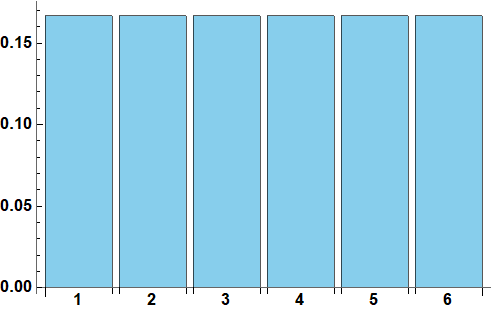
When you roll a single die, you get a number from the set $\{1,2,3,4,5,6\}$, each with an equal probability of $1/6$. There's nothing remotely bell-shaped about this—it's flat, symmetric, and completely uniform across six outcomes. No hint of a Gaussian curve here. But things will change as we add more dice.
In this post, we'll build intuition for the Central Limit Theorem by starting with something concrete; rolling dice. We'll begin with single and multiple tosses, introduce a clever algebraic tool to count outcomes, derive a closed-form formula for the distribution, and finally show how the familiar bell curve naturally arises in the limit of many rolls.
Rolling two dies
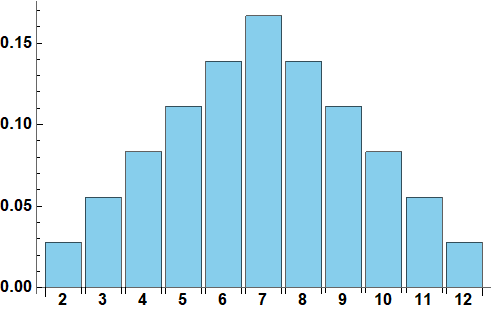
Now, let's roll two dice instead. This time, we add the two numbers we roll together. (Rolling one die twice is basically the same idea - the important part is independence of individual throws). What numbers can we get? Since each die shows a value between 1 and 6, their sum can range from 2 to 12.
But the important thing is: not all sums are equally likely. For example, there's only one way to get a 2 (rolling 1 and 1), but there are several ways to get a 7 (like 1+6, 2+5, 3+4, etc.).
Why? Because we're summing two independent variables. Each possible combination (1–6 for each die) is equally likely, but their sums cluster around the middle values more often.
Here's a breakdown:
| Sum | Ways to get it | Probability |
|---|---|---|
| 2 | (1,1) | 1/36 |
| 3 | (1,2), (2,1) | 2/36 |
| 4 | (1,3), (2,2), (3,1) | 3/36 |
| 5 | (1,4), (2,3), (3,2), (4,1) | 4/36 |
| 6 | (1,5), (2,4), (3,3), (4,2), (5,1) | 5/36 |
| 7 | (1,6), (2,5), (3,4), (4,3), (5,2), (6,1) | 6/36 |
| 8 | (2,6), (3,5), (4,4), (5,3), (6,2) | 5/36 |
| 9 | (3,6), (4,5), (5,4), (6,3) | 4/36 |
| 10 | (4,6), (5,5), (6,4) | 3/36 |
| 11 | (5,6), (6,5) | 2/36 |
| 12 | (6,6) | 1/36 |
We can neatly visualize the probability mass function (PMF) for the sum of two dice like this:
Now, one might wonder: are we doomed to manually count the number of possibilities for each outcome whenever we want to bring in more dice? Well, yes and no. Ideally, we'd like a formula that gives us, for the number of dice $n$ and a possible outcome $k$, the number of possibilities $N(k; n)$, or the probability $p(k; n) = N(k; n) / (6^n)$. To do that, we use a cute little math trick.
Dice tosses: formula for probability
This trick uses polynomials to sort out the possible outcomes of dice tosses. First, notice that multiplying two terms, each in the form $x^{\text{some power}}$, simply causes the powers to add:
$$ x^a x^b = x^{a + b} $$
Multiplying powers of $x$ adds exponents. So $x^3 \cdot x^5 = x^8$ symbolically corresponds to rolling a 3 and a 5 and summing the result.
$$ P_1(x) \equiv x^1 + x^2 + x^3 + x^4 + x^5 + x^6 $$
In a sense, this polynomial hides all possible outcomes of a single die toss in its terms. How about tossing two dice? We simply multiply two copies of this polynomial. Here's the neat part: when we multiply these polynomials, the coefficient of each $x^k$ in the expansion tells us how many ways we can get a sum of $k$ from $n$ dice.
The numbers 1, 2, 3, ... we see here are exactly the number of ways to achieve sums of 2, 3, 4, ... ! When we expand the polynomials and group together terms with the same power of $x$, the prefactor corresponds to the number of ways that power appears in the product. This gives us the general expression:
In other words, the frequencies $N (k; n)$ appear as the coefficients of the expansion of the function $P_n (x)$,
$$ P_n (x) = \sum_{k = n}^{6n} N (k; n) x^k $$
In this sense, $P_n (x)$ is the generating function of our frequency coefficients of $n$ dice toss sum. To move towards a more useful formula, we now look at the expression $P_1 (x)$ again. To simplify $P_1(x)$, we factor it to a more useful form. This lets us handle large powers more elegantly. We start by taking out a common factor of x
$$ P_1 (x) = x \left( 1 + x + x^2 + x^3 + x^4 + x^5 \right) $$
Now we use a well known fact about polynomial series to simplify the expression $S \equiv 1 + x + \cdots + x^5$ (or other general power, since the logic is not dependent on the last coefficient being specifically $x^5$). We compare $S$ and $x S$:
$$ \begin{aligned} S &= 1 + x + x^2 + x^3 + x^4 + x^5 \\ x S &= x + x^2 + x^3 + x^4 + x^5 + x^6 \end{aligned} $$
We see, that the two differ only by the first term in $S$ (1) and last term in $x S$ ($x^6$). Thus, their difference is
Going back to the generating function $P_n (x)$, we now see
$$ P_n (x) = \left( P_1 (x) \right)^n = x^n \left( \frac{1 - x^6}{1 - x} \right)^n $$
The reason we brought the generating function to this form is that the resulting expansion is somewhat simpler than using the multinomial theorem on the sum $1 + x + \cdots + x^5$. We now need to expand all pieces of $P_n$ and put them together. We start with the denominator, which is given by a simple geometric series
$$ \frac{1}{1 - x} = \sum_{j = 0}^\infty x^j = 1 + x + x^2 + \cdots $$
Luckily, the $n$-th power of this series can be handled by using derivatives instead of a complicated multinomial expansion. First, we notice a pattern
$$ \begin{aligned} \frac{\mathrm{d}}{\mathrm{d} x} \frac{1}{1 - x} &= \frac{1}{(1 - x)^2} \\ \frac{\mathrm{d}}{\mathrm{d} x} \frac{1}{(1 - x)^2} &= \frac{2}{(1 - x)^3} \\ \frac{\mathrm{d}}{\mathrm{d} x} \frac{1}{(1 - x)^3} &= \frac{2 \cdot 3}{(1 - x)^4} \\ \frac{\mathrm{d}}{\mathrm{d} x} \frac{1}{(1 - x)^4} &= \frac{2 \cdot 3 \cdot 4}{(1 - x)^5} \end{aligned} $$
From this pattern, we can generalize (proof left as a gentle exercise for the reader):
Let's unleash this on our geometric series. We know, that due to the $n-1$ derivatives with respect to $x$, the first non-vanishing term in the geometric series will be $x^{n - 1}$
Notice, that the term in the last expression is equivalent to the following binomial coefficient
$$ \frac{(n + j - 1)!}{(n-1)! \; j!} = \binom{n + j - 1}{n - 1} $$
Now we express the numerator $(1 - x^6)^n$ in terms of a sum using binomial theorem
$$ (1 - x^6)^n = \sum_{\ell = 0}^n (-1)^\ell \binom{n}{\ell} x^{6 \ell} $$
Finally, putting everything together,
$$ P_n (x) = x^n \sum_{j = 0}^\infty \binom{n + j - 1}{n - 1} x^j \sum_{\ell = 0}^n (-1)^\ell \binom{n}{\ell} x^{6 \ell} $$
Now that we've derived the full expansion, we can finally extract the coefficient of $x^k$, giving us the number of ways to get the sum $k$ with $n$ dice. For a given $n \leq k \leq 6n$, the coefficient of $x^k$ in $P_n (x)$ is given by a condition $n + j + 6 \ell = k$, from which we can fix $j$ and thus get rid of one of the sums
$$ N (k;n) = \sum_{\ell = 0}^{\ell_{\text{max}}} (-1)^\ell \binom{k - 6 \ell - 1}{n - 1} \binom{n}{\ell} $$
The upper limit of this sum can be fixed by demanding that $k - 6 \ell - 1 \geq n - 1$, and thus $\ell \leq (k - n) / 6$. If $(k - n) / 6$ is not an integer, then the upper limit is given by the largest integer not exceeding $(k - n) / 6$, i.e. the floor of $(k - n) / 6$, $\ell_{\text{max}} = \lfloor (k - n) / 6 \rfloor$.
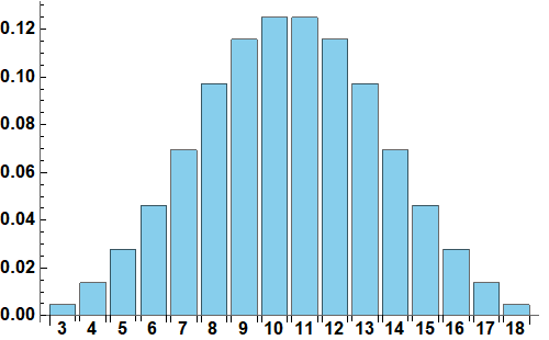
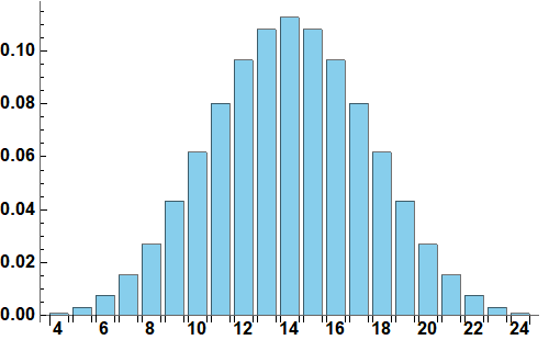
We can now use our new formula for $N(k;n)$ to find the probability distribution for $n = 3, 4, ...$
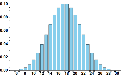
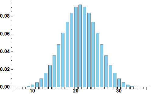
Many, many dice tosses: marching towards the Gaussian limit
While elegant, this formula isn't very helpful when $n$ becomes large. Summing over so many terms quickly becomes tedious. So how do we handle thousands of dice tosses? We need to zoom out—to stop caring about exact numbers and start looking at the big picture. That's where normalization and limiting behavior come in. First, we introduce a modified random variable, $y$, that is corrected for the mean and standard deviation in $N (k; n)$. The mean is simple; we know, that the mean value of the outcome of $n$ dice is $((1 + 6) / 2) n = (7/2) n$. As for the variance, we recall our generating function for $N (k; n)$ and how it relates to the probability distribution
$$ P_n (x) = \sum_{k = n}^{6n} N (k; n) x^k $$
Using $p (k; n) = N (k; n) / 6^n$ to rewrite the above expression for probability instead of frequency, we find
$$ G_n (x) \equiv \frac{1}{6^n} P_n (x) = \sum_{k = n}^{6n} p (k; n) x^k = \left\langle x^k \right\rangle $$
where we realized that the sum over probabilities corresponds to a certain, special, parametric, mean value (here $x$ is the parameter, while $k$ is a random variable we sum over). That's right, the function $G_n (x)$ corresponds to the probability-generating function of the dice toss distribution! Knowing this, we can calculate various expectation values (average quantities). For example, we already know that all probabilities should sum up to 1, but still,
What about the mean value? We need to calculate the following sum:
$$ \left\langle k \right\rangle = \sum_{k = n}^{6n} p (k; n) \, k $$
But our original probability-generating function contains terms $x^k$, not $k$. However, we can use the following neat derivative trick:
$$ \frac{\mathrm{d}}{\mathrm{d} x} x^k = k x^{k-1} \quad \to \quad k = \left. \frac{\mathrm{d}}{\mathrm{d} x} x^k \right|_{x = 1} $$
We can now apply this to the probability-generating function. Since the sum is finite, we can just differentiate it term by term (note - the coefficients do not contain $x$, so the derivative passes through them like Taco Bell passes through my digestive track on Friday evening) and obtain
At this point, we can replace the sum with the probability-generating function and get
$$ \left\langle k \right\rangle = \left. \frac{\mathrm{d}}{\mathrm{d} x} G_n (x) \right|_{x = 1} = G_n^\prime (1) $$
Now, what is $G_n^\prime (1)$? Glad you asked, calculating mean values was never easier:
Putting back the factor $1 / 6^n$, we get
$$ \mu = \left\langle k \right\rangle = \frac{21 \cdot 6^{n - 1}}{6^n} n = \frac{21}{6} n = \frac{7}{2} n $$
as expected. Now that we know the method works, we can calculate another mean required for variance; $\langle k^2 \rangle$. To do that, we use derivatives again. First, we express $k^2$ in terms of $x^k$ as follows
This time, the calculation gives us variance (left as a homework exercise for your favorite algebra software)
$$ \sigma^2 = \left\langle k^2 \right\rangle - \left\langle k \right\rangle^2 = \frac{35}{12} n $$
Now, let's define a normalized random variable
$$ y = \frac{k - \mu}{\sigma} $$
Normalized dice toss statistics
Our goal is to figure out the probability density function (PDF) of $y$ in the limit of large $n$. While the variable $k$ is discrete (only having integer values), in the limit of large $n$, variable $y$ becomes "more and more continuous", to the point we can speak of a probability distribution, instead of a probability mass function. In the next part of the series we will prove this result for any random process, but for now, we will use the probability-generating function we derived earlier
We will now normalize the distribution to zero mean and unit variance. We already found that the original distribution $p (k; n)$ has mean $\mu = 7n / 2$ and variance $\sigma^2 = 35 n / 12$. Changing $k \to k^\prime = \sigma \, k + \mu$ and $p (k;n) \to \sigma \, p (k^\prime ; n)$ normalizes the distribution. For a linear transformation, it can be easily shown that the probability-generating function transforms as follows
Now we want to show the limit $n \to \infty$, which becomes significantly easier if we show it for $\log G_n (x)$ rather than $G_n (x)$ itself. Logarithm of the transformed $G_n (x)$ reads
To obtain the limit when $n \to \infty$, we can replace $t = 1 / n$ and use Taylor series. A tricky calculation later (given as a homework to a bored reader) reveals
All right—so far we've expanded the probability-generating function and seen that it reduces to a single term as $n$ increases. But does its corresponding distribution really converge to a Gaussian? To show that it does, we need to compute $\log G_{\mathcal{N}} (x)$ for the perfect Gaussian and show it is equivalent to the first term in our expansion. This is a matter of a simple integral and completing the square
$$ \begin{aligned} G_\mathcal{N} (x) &= \frac{1}{\sqrt{2 \pi}} \int \limits_{-\infty}^\infty \mathrm{d} u \, x^u \, \exp \left( - \frac{u^2}{2} \right) = \\ &= \frac{1}{\sqrt{2 \pi}} \int \limits_{-\infty}^\infty \mathrm{d} u \, \exp \left( - \frac{u^2}{2} + u \log x \right) = \\ \frac{1}{\sqrt{2 \pi}} &\int \limits_{-\infty}^\infty \mathrm{d} u \, \exp \left[ - \frac{1}{2} \left( u - \log x \right)^2 + \frac{\log^2 x}{2} \right] = \\ &= \exp \left( \frac{\log^2 x}{2} \right) \end{aligned} $$
which is, after applying logarithm, exactly the first term of the expansion of $G_n (x)$ for large $n$.
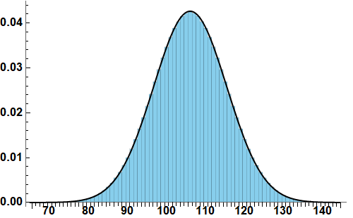
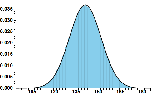
As we can see, the limit $n \to \infty$ truly converges towards a perfect Gaussian. We can check the histograms for actual dice tosses for larger $n$ and see that the process converges really quickly (here I also added the corresponding Gaussian curve for comparison):
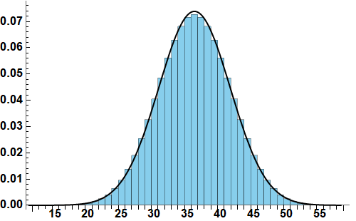
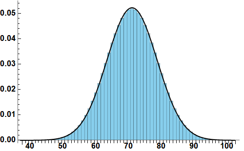
Conclusion: why the bell curve appears
We've seen that even something as simple as rolling dice already contains the seeds of the Gaussian. As the number of dice increases, the distribution of their normalized sum smoothly morphs into a bell curve. This is the Central Limit Theorem at work: the average of many independent, finite-variance variables converges to the normal distribution.
In the next post, we'll explore how this logic extends to continuous processes, and why the Gaussian remains such a dominant force in probability, statistics, and physics.
Bonus: this whole analysis can be repeated for a $s$-sided coin. If you wonder whether the convergence to a Gaussian is faster or slower, it's neither; changing the number of sides barely changes anything about the speed of convergence. The coefficients next to $t^4$ and $t^6$ can be obtained through expansion:
$$ \begin{aligned} &\frac{1}{8} - \frac{s^2 + 1}{s^2 - 1} \frac{1}{n} \\ &\frac{1}{48} + \frac{s^2 + 1}{40 (s^2 - 1)} \frac{1}{n} - \frac{s^4 + s^2 + 1}{105 (s^2 - 1)^2} \frac{1}{n^2} \end{aligned} $$
and as you can see, increasing $s$ has very little effect on the size of the terms containing $n$. Thus, increasing the number of sides on a dices has virtually no effect on the speed of the convergence towards a Gaussian.