See Why Gaussian? Part I: tossing dice for part 1!

See Why Gaussian? Part II: continuous additive processes for part 2!

In the first part of this series, we saw how a discrete random variable (like a roll of a die), when accumulated across independent trials, converges toward a Gaussian distribution. In the second part, we extended this to continuous variables - showing how, under mild conditions on their moments, the same convergence occurs.

In this post, we take a different path. Not all natural processes are additive. Some involve multiplication, cyclic variables, or nonlinear transformations. Yet, remarkably, the Gaussian often still emerges-sometimes not in the variable itself, but in a transformed version like its logarithm or phase. Let's explore these less-obvious routes to Gaussian behavior.

Multiplicative random processes

While the central limit theorem is traditionally associated with additive processes, many real-world systems operate multiplicatively. Fortunately, multiplication becomes addition in logarithmic space, so a wide array of CLT-like results still apply, just one transformation away. In fact, many systems that produce log-normal statistics are fundamentally multiplicative at their core.

Consider a few well-known examples: compound interest in finance, population growth with random fluctuations, or the cascade of returns in stock markets - all evolve by repeated multiplication of random factors. In such cases, taking the logarithm converts the product into a sum, and the central limit theorem applies to the log-transformed variable. As a result, the original variable becomes log-normally distributed.

One particularly elegant example comes from astrophysical fluid dynamics: the density structure in isothermal, supersonic turbulence. In such flows, density fluctuations are largely governed by shock waves. Each shock compresses the local density by a factor determined by the velocity field, so the density doesn't evolve additively, but multiplicatively. For isothermal shocks (where the adiabatic index $\gamma = 1$), the Rankine–Hugoniot jump condition simplifies to a density jump $\rho_2 / \rho_1 = m^2$, where (dimensionless) $m$ is the upstream Mach number; the speed of the shock reduced by the speed of sound. As gas elements traverse a sequence of shocks, the resulting density is repeatedly multiplied by factors drawn from the local velocity dispersion. To be clear, if a parcel of gas is affected by $n$ shocks passing through it, each propagating with some random local Mach number $m$, the resulting density will be

$$ \rho = \rho_0 \, m_1 \, m_2 \cdots m_n $$

Naturally, to understand the distribution of final densities, we must know how the local Mach number itself is distributed. In a turbulent flow, these are not fixed, but fluctuate based on the local velocity field. The precise form of the Mach number distribution depends on the turbulence driving and thermodynamic conditions, but it's generally broad and continuous, with most values clustered near the mean turbulent Mach number.

If we assume the Mach numbers $m_i$ for each shock are drawn independently from such a distribution (or more realistically, weakly correlated), then the logarithm of the final density becomes a sum of random terms:

$$ \log (\rho / \rho_0) + \log m_1 + \log m_2 + \cdots + \log m_n. $$

This is precisely the setup where the central limit theorem applies. Under fairly weak assumptions about the shape and variance of the $\log m$ distribution, the sum converges toward a Gaussian. Therefore, the logarithm of density, $s \equiv \log (\rho / \rho_0)$ follows a normal distribution, and the density itself follows a lognormal distribution:

$$ f (s) \sim \mathcal{N}(\mu, \sigma^2), \quad \text{so} \quad f (\rho) \sim \frac{1}{\rho} \exp\left(-\frac{(\log (\rho / \rho_0) - \mu)^2}{2\sigma^2} \right). $$

$$ f (s) \sim \mathcal{N}(\mu, \sigma^2) $$

so,

$$ f (\rho) \sim \frac{1}{\rho} \exp\left(-\frac{(\log (\rho / \rho_0) - \mu)^2}{2\sigma^2} \right) $$

But what does the distribution of local Mach numbers actually look like in a turbulent flow? Since the Mach number $m = v / c_s$ is just the velocity normalized by the sound speed, this really comes down to the statistics of local velocity magnitudes.

In an isothermal turbulent medium with no large-scale bulk motion, the three Cartesian components of velocity can be reasonably modeled as independent random variables drawn from a Gaussian distribution centered at zero-thanks to the central limit effect of countless random driving forces. When this is the case, the magnitude of the velocity (and hence the local Mach number) follows a Maxwell–Boltzmann distribution.

In three dimensions, the Maxwellian PDF for the Mach number $m$ takes the form:

$$ f (m) = \frac{4 \pi m^2}{(2 \pi \sigma^2)^{3/2}} \exp \left( - \frac{m^2}{2 \sigma^2} \right) $$

where $\sigma$ is the standard deviation of the underlying 1D velocity components (in units of the sound speed). This shape arises naturally when you compute the distribution of the magnitude of a 3D Gaussian vector. Most of the probability mass lies around the typical turbulent Mach number, but there's a non-negligible tail at high $m$, allowing for occasional strong shocks.

There's one important complication we need to address before we go further: real shock waves only occur when the flow is supersonic, that is, when the Mach number $m > 1$. If the flow is subsonic, information travels fast enough upstream to smooth out any discontinuity before a shock can form. In our setup, however, we're drawing Mach numbers from a continuous distribution (like the Maxwellian), which includes both subsonic and supersonic values.

So what happens to those subsonic samples in our model? Strictly speaking, they shouldn't correspond to shocks at all. But in turbulent flows, not every compressive or expansive feature is a perfect shock. There are also rarefaction waves, which are smooth expansions rather than discontinuous jumps. Unlike shocks, which compress the gas and increase the density, rarefactions decrease the density across a smooth gradient.

In our simplified picture, we can treat these rarefactions as "anti-shocks"; they still change the density by a multiplicative factor, but one that's less than one. A convenient way to model both compression and expansion statistically is to let each event (shock or rarefaction) multiply the density by a factor of $m^2$, even when $m < 1$. This may not match every microscopic detail, but it captures the essential multiplicative character of density evolution in turbulent media.

This Maxwellian form gives us a physically motivated, continuous distribution from which to draw the multiplicative shock factors $m^2$. With that foundation in place, we're finally ready to run a small numerical experiment.

Shocks as a random multiplicative process: numerical experiment

We'll simulate a parcel of gas undergoing a series of random isothermal shocks. Each shock multiplies the current density by $m^2$, where the Mach number $m$ is drawn from the Maxwellian distribution with some pre-defined $\sigma$. After a few such multiplicative steps, we'll examine the distribution of the resulting density.

Here's a Python code that will give us some distributions:

import numpy as np
import matplotlib.pyplot as plt
from scipy.stats import maxwell, norm, lognorm
from tqdm import tqdm
import os

import numpy as np
import matplotlib.pyplot as plt
from scipy.stats import maxwell, norm, lognorm
import os

def multiplicative_clt_demo(
    n=5,
    N=10000,
    bins=100,
    base_dir="",
    title="Multiplicative CLT Demo",
    filename="lognormal_plot.png",
    sigma=2.0,
    toggle_gaussian=True,
    toggle_lognormal=True,
    threshold=0.005
):
    # sample mach numbers from maxwellian
    log_density = np.zeros(N)
    for _ in tqdm(range(n), desc="Applying shocks", ascii=True):
        mach = maxwell.rvs(scale=sigma, size=N)
        log_density += 2 * np.log(mach)  # because shock_factors = mach^2

    # normalize the ensemble towards zero mean and unit variance
    mu = np.mean(log_density)
    std = np.std(log_density)
    log_density_norm = (log_density - mu) / std

    # we also need density for plotting
    density = np.exp(log_density_norm)
    mu = 0
    std = 1

    # --- LOG-DENSITY PLOT ---
    plt.figure(figsize=(8, 5))
    counts, bin_edges = np.histogram(log_density_norm, bins=bins, density=True)
    bin_width = bin_edges[1] - bin_edges[0]
    bin_centers = bin_edges[:-1]

    plt.bar(
        bin_centers, counts, width=bin_width,
        color="skyblue", edgecolor="none",
        align="edge", label="Normalized log-density")
    for x, height in zip(bin_centers, counts):
        plt.plot([x, x + bin_width], [height, height],
        color="black", linewidth=0.5)

    if toggle_gaussian:
        significant = counts > threshold * np.max(counts)
        x_min = bin_edges[np.argmax(significant)]
        x_max = bin_edges[::-1][np.argmax(significant[::-1])]
        x_range = x_max - x_min
        x = np.linspace(x_min - 0.1 * x_range, x_max + 0.1 * x_range, 1000)
        y = norm.pdf(x, loc=0, scale=1)
        plt.plot(x, y, 'k--', label="Ideal Normal Distribution")

    plt.title(f"{title}\nLog-density (n={n}, N={N}, σ={sigma})")
    plt.xlabel("Normalized log-density")
    plt.ylabel("Probability Density")
    plt.grid(True)
    plt.legend(loc="upper right")
    plt.ylim(top=max(counts.max(), y.max() if toggle_gaussian else 0) * 1.2)
    plt.xlim(x[0], x[-1])

    path_log = os.path.join(base_dir, "log_" + filename)
    plt.savefig(path_log, dpi=150)
    plt.close()
    print(f"Saved log-density plot to {path_log}")

    # --- DENSITY PLOT ---
    plt.figure(figsize=(8, 5))

    # Fix histogram x-axis range
    density_min = 0
    density_max = 10  # adjust as needed

    # Manually define bin edges and bin centers
    bin_edges_d = np.linspace(density_min, density_max, bins + 1)
    bin_width_d = bin_edges_d[1] - bin_edges_d[0]
    bin_centers_d = bin_edges_d[:-1]

    # Clip data to range
    density_clipped = density[
        (density >= density_min) &
        (density <= density_max)]
    counts_d, _ = np.histogram(density_clipped,
        bins=bin_edges_d, density=True)

    # Plot bars
    plt.bar(
        bin_centers_d,
        counts_d,
        width=bin_width_d,
        color="lightcoral",
        edgecolor="none",
        align="edge",
        label="Density"
    )

    for x, height in zip(bin_centers_d, counts_d):
        plt.plot([x, x + bin_width_d], [height, height],
        color="black", linewidth=0.5)

    # Overlay lognormal
    if toggle_lognormal:
        x_d = np.linspace(density_min, density_max, 1000)
        y = lognorm.pdf(x_d, s=std, scale=np.exp(mu))
        plt.plot(x_d, y, 'k--', label="Ideal Lognormal Distribution")

    # Finalize plot
    plt.title(f"{title}\nDensity (n={n}, N={N}, σ={sigma})")
    plt.xlabel("Density")
    plt.ylabel("Probability Density")
    plt.grid(True)
    plt.legend(loc="upper right")
    plt.ylim(top=max(counts_d.max(), y.max() if toggle_lognormal else 0) * 1.2)
    plt.xlim(density_min, density_max)

    # Save
    path_density = os.path.join(base_dir, "density_" + filename)
    plt.savefig(path_density, dpi=150)
    plt.close()
    print(f"Saved density plot to {path_density}")

for n in [1, 2, 3, 4, 5, 10, 20, 30, 40, 50, 100, 200, 300, 400, 500]:
    multiplicative_clt_demo(
        n=n,
        N=10000000,
        bins=200,
        base_dir="CLT_plots",
        title="Multiplicative Central Limit Theorem",
        filename="mach_lognormal_n" + str(n) + ".png",
        sigma=2.0
    )

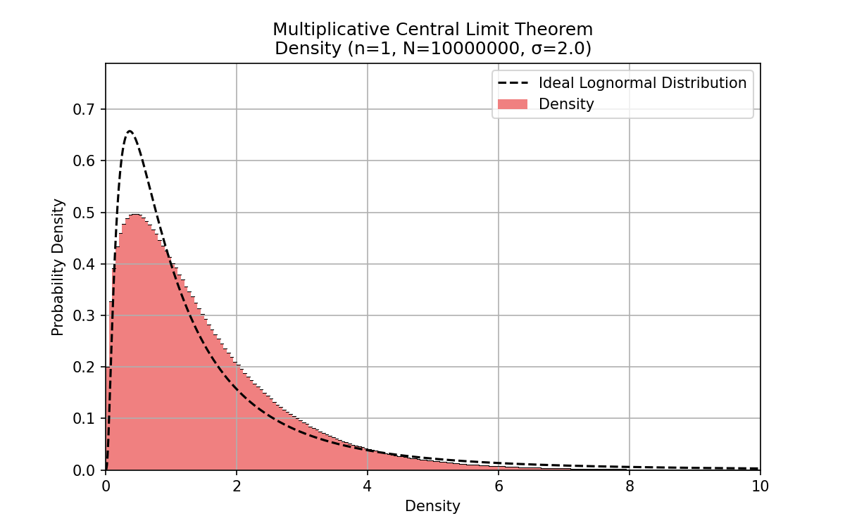
Let's watch how the distribution of density converges to the ideal lognormal distribution as the number of shocks $n$ increases:

And now let's see the same effect in the logarithmic space:

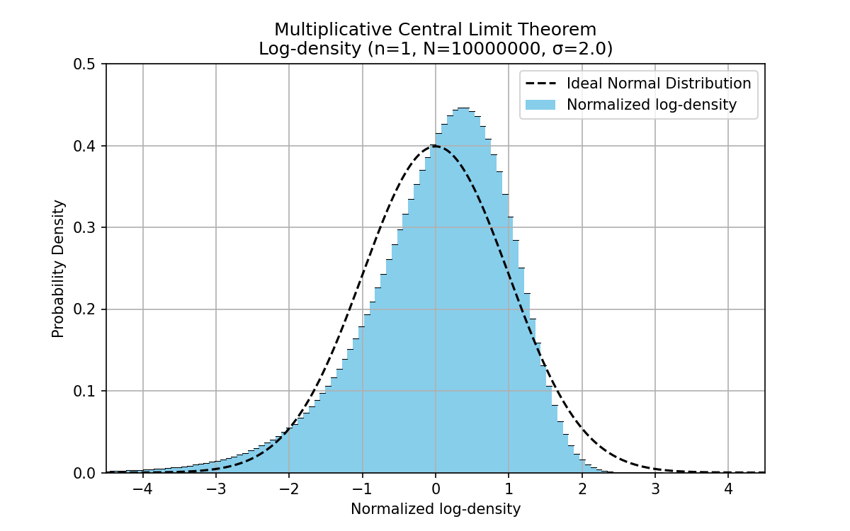
We see that while the convergence happens, it happens quite slow; we will see shortly why.

Analytic exploration

We saw that when $n$ is low, starting from $n = 1$, the resulting distribution for $s = \log (\rho / \rho_0)$ is heavily skewed to the right. Increasing $n$ makes the distribution for $s$ converge to the standard Gaussian, but it does so slowly - visible deviations persist even for large $n$, such as $n = 100$. This is exactly what we'd expect based on the results derived in Part II: a finite, nonzero third moment in the source distribution leads to convergence at a rate of $1/\sqrt{n}$.

In fact, the distribution of the logarithm of the Mach number squared - i.e., the fundamental building block in our multiplicative model - is significantly skewed. Its right tail decays exponentially, while the left tail only falls off quadratically. Since the $n = 1$ case directly samples from this source distribution its asymmetry is immediately visible. Let's now explore this analytically.

We begin by introducing a change of variables. Let the shock Mach number $m$ follow a Maxwellian distribution:

$$ f_M(m) = \frac{4 \pi m^2}{(2 \pi \sigma^2)^{3/2}} \exp\left( -\frac{m^2}{2\sigma^2} \right), $$

where $\sigma$ is the one-dimensional velocity dispersion (in units of sound speed). We now define a new variable $y = \log(m^2)$. This transformation gives:

$$ m = e^{y/2}, \quad \frac{dm}{dy} = \frac{1}{2} e^{y/2}. $$

The distribution of $y$ can be obtained by a simple variable transform

$$ f_Y(y) \, \mathrm{d} y = f_M (m) \, \mathrm{d} m \quad \implies \quad f_M(m(y)) \left| \frac{dm}{dy} \right| = \frac{1}{\sqrt{2\pi} \sigma^3} e^{\frac{3y}{2}} \exp\left( -\frac{e^y}{2 \sigma^2} \right). $$

$$ \begin{aligned} f_Y(y) \, \mathrm{d} y &= f_M (m) \, \mathrm{d} m \; \implies \; f_M(m(y)) \left| \frac{dm}{dy} \right| = \\ &= \frac{1}{\sqrt{2\pi} \sigma^3} e^{\frac{3y}{2}} \exp\left( -\frac{e^y}{2 \sigma^2} \right). \end{aligned} $$

This is the exact shape of the log-distribution from which each shock multiplicative factor is drawn. While it superficially resembles a lognormal, it is not symmetric and possesses significant skewness. To explore this in more detail, we can compute its moments.

From this, we can compute the central moments analytically. The mean of $y$ is:

$$ y_0 \equiv \langle y \rangle = 2 - \gamma - \log 2 + 2 \log \sigma, $$

where $\gamma \approx 0.5772$ is the Euler–Mascheroni constant. The variance is:

$$ \Sigma^2 = \left\langle (y - y_0)^2 \right\rangle = \frac{1}{2} (\pi^2 - 8), $$

and the third central moment is:

$$ \left\langle (y - y_0)^3 \right\rangle = 2(8 - 7\zeta(3)) \approx -0.8288, $$

which confirms the heavy negative skew we observed in our numerical experiments. More specifically, Fischer's coefficient of skewness relates the third central moment to the standard deviation:

$$ \bar{\mu}_3 = \frac{\left\langle (y - y_0)^3 \right\rangle}{\Sigma^3} \approx -0.9170 $$

Indicating a high negative skewness. Importantly, these moments - particularly the variance and skewness - are independent of $\sigma$. The only effect of $\sigma$ is to shift the distribution along the $y$-axis. In other words, the strength of the turbulence affects the mean density in log-space, but not the statistical structure of the fluctuations.

This has a deep implication: the convergence of $s = \log \rho$ to a Gaussian is governed by a universal source distribution whose shape is unaffected by the Mach number. The only thing turbulence strength (through $\sigma$) does is translate the curve - it does not change how skewed or wide it is. Thus, in this model, the physics of the turbulence gets “washed out” in the fluctuation statistics, leaving behind a shape that is universal and determined entirely by the structure of the multiplicative process.

To obtain the distribution for some specific $n$, we employ the characteristic function again, starting from the characteristic function of the underlying Maxwellain in the log-space. First, we normalize the distribution to zero mean and unit variance by subtracting and rescaling the random variable $y \to \Sigma (y - y_0)$:

$$ f_Y (y) = \frac{\Sigma}{\sqrt{2 \pi}} \exp \left( \frac{3 \Sigma}{2} (y + y_0) - \frac{1}{2} e^{\Sigma (y + y_0)} \right) $$

where we can take $\sigma = 1$ without the loss of generality, since we already established that the overall shape does not depend on $\sigma$. Our task is now to obtain the characteristic function $\phi_y (t) = \langle e^{i t y} \rangle$. This means we have to calculated the following integral:

$$ \phi_y (t) = \int \limits_{- \infty}^{\infty} \mathrm{d} y \, e^{i t y} f_Y (y) $$

This integral can be performed analytically (using substitution $u = (1/2) e^{\Sigma y}$ and the integral definition of Gamma function/factorial) and the result is:

$$ \phi_y (t) = \left( 4 e^{\gamma - 2} \right)^{i t / \Sigma} \frac{2}{\sqrt{\pi}} \Gamma \left( \frac{3}{2} + \frac{i t}{\Sigma} \right) $$

As we saw before, the characteristic function of log-density $s = (y_1 + \cdots + y_n) / \sqrt{n}$ thus is:

$$ \phi (t; n) = \left( \phi_y (t / \sqrt{n}) \right)^n = \left( 4 e^{\gamma - 2} \right)^{\sqrt{n} i t / \Sigma} \left[ \frac{2}{\sqrt{\pi}} \Gamma \left( \frac{3}{2} + \frac{i t}{\sqrt{n} \Sigma} \right) \right]^n $$

$$ \begin{aligned} \phi (t; n) &= \left( \phi_y (t / \sqrt{n}) \right)^n = \\ = \left( 4 e^{\gamma - 2} \right)^{\sqrt{n} i t / \Sigma} &\left[ \frac{2}{\sqrt{\pi}} \Gamma \left( \frac{3}{2} + \frac{i t}{\sqrt{n} \Sigma} \right) \right]^n \end{aligned} $$

From which the PDF of $s$ can be obtained by the inverse Fourier transform:

$$ f(s; n) = \frac{1}{2 \pi} \int \limits_{-\infty}^{\infty} \mathrm{d} t \, e^{- i t s} \phi (t; n) $$

Unfortunately, for a general value of $n$ the result cannot be expressed via any known functions. Nevertheless, we can obtain the distribution numerically and plot the results:

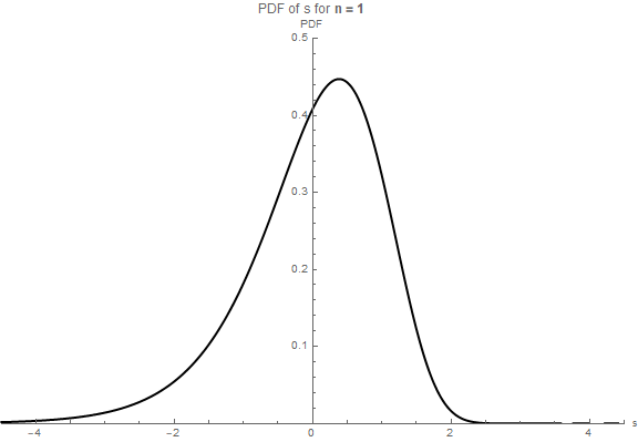
This construction not only confirms that the central limit behavior applies to a sequence of multiplicative shocks in log-space, but also provides a concrete route to compute the resulting distribution of log-density for any finite number of events. In particular, the characteristic function formalism highlights the slow convergence to Gaussianity when the underlying distribution is skewed - as is the case here, due to the asymmetric shape of the Maxwellian in logarithmic coordinates.

More analytical results and applications of this model can be found in our paper Rabatin & Collins (2022), which this post is based on.