April 29, 2025
Why Gaussian? Part II: continuous additive processes
See Why Gaussian? Part I: tossing dice for part 1!
See Why Gaussian? Part III: not all processes are additive for part 3!
In the first part on this topic, Why Gaussian? Part I: tossing dice, we explored how tossing more and more dice and summing the result of all tosses gives us a number that's distributed closer and closer to a Gaussian. In the second part, we will observe the same thing happening for continuous processes, where the underlying numbers come from a distribution over real numbers (or a continuous interval).
We start by defining a source distribution - it can be anything not too pathological (it should have well-defined mean and variance), $\mathcal{D} (x)$. We can verify the CLT for a process, in which we don't get a number directly from the source distribution, rather, we get an average of $n$ values generated by this random process
$$ X = \frac{1}{n} \sum_{i = 1}^n x_i, \quad x_i \sim \mathcal{D} $$
We will see, that value $X$ follows a distribution closer and closer to Gaussian if $n$ is large. We will see this by taking an ensemble of $N$ samples $(X_1, X_2, \dots, X_N)$. Since the overall mean and variance might, over many samples $n$, drift far away from the origin (especially if the source distribution does not have zero mean), we renormalize the samples by subtracting the ensemble mean and dividing by variance:
Now we (or rather the central limit theorem) claim that the distribution of $Y_k$ will tend to the normal distribution if $n$ is large enough. Let's verify this using Python! We start by importing all the required modules:
import numpy as np
import matplotlib.pyplot as plt
import os
Here numpy is required to generate the random samples, matplotlib for making neat plots and os for I/O. Having done that, we now proceed with the function that will generate the samples, renormalize them, create histograms and save the histograms. Thinking ahead, we know we will need several inputs: the random distribution, $n$, $N$. Additionally, we will also control the number of bins to create the resulting distribution. We can include more arguments to make plotting more modular, but ultimately, the core of the function is captured with the first 4 arguments.
def clt_demo(
    dist_func, # source random distribution
    n=5, # baseline number of random variables to sum
    N=10000, # size of the ensemble
    bins=50, # number of bins for visualization
    base_dir="",
    title="CLT Demo",
    filename="plot.png"
    bounds=[-10,10] # cutoff if the distribution is weird
):
The neat thing about Python is its vectorization capabilities; almost all built-in functions are capable of taking in an array of arbitrary shape which then results in output of the same shape, where the function is applied to each element. We can utilize this by generating $N \times n$ values all at once in a big $N \times n$ array, which we then sum over the last index. Specifically,
samples = dist_func(size=(N, n))
sums = np.sum(samples, axis=1)
For really high $n$ and $N$, we would implement a different strategy where the sum is being performed on the fly to save the memory. Having done this, the rest of the code simply normalizes the ensemble, plots the histogram and saves it. Full code with some examples:
We can now look at some examples. We start with the uniform baseline distribution that generates numbers between 0 and 1 with equal probability. With that, the expected histogram for $n = 1$ is flat:
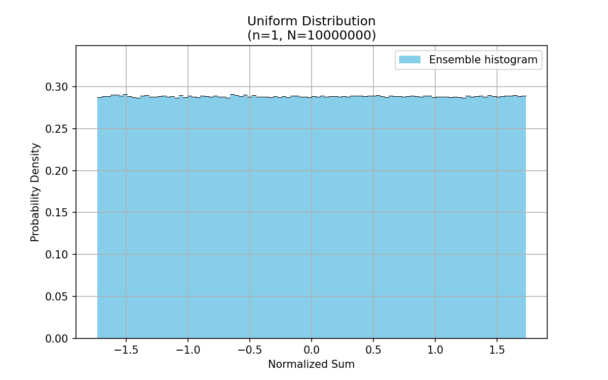
The range changed due to the normalization to zero mean and unit variance. Now, if we increase $n$ to $2, 3, 4, 5$, we get closer and closer to the Gaussian distribution:
Convergence towards a distribution is a very rich and interesting topic; not all distributions will lead to the Gaussian; a heavy-tailed Cauchy distribution will converge to another Cauchy distribution, for example. However, as long as the distribution is "well-behaved", convergence is assured. Berry-Esseen's theorem guarantees a relatively slow convergence (the difference between Gaussian and the distribution after summing $n$ terms is on the order of $1/\sqrt{n}$) provided the third moment $\langle x^3 \rangle$ exists and is finite. We saw that the convergence for the uniform distribution is rather quick; this is because the third moment is actually zero, in which case the convergence is slightly faster ($1/n$). The behavior for the Cauchy distribution can be observed here:
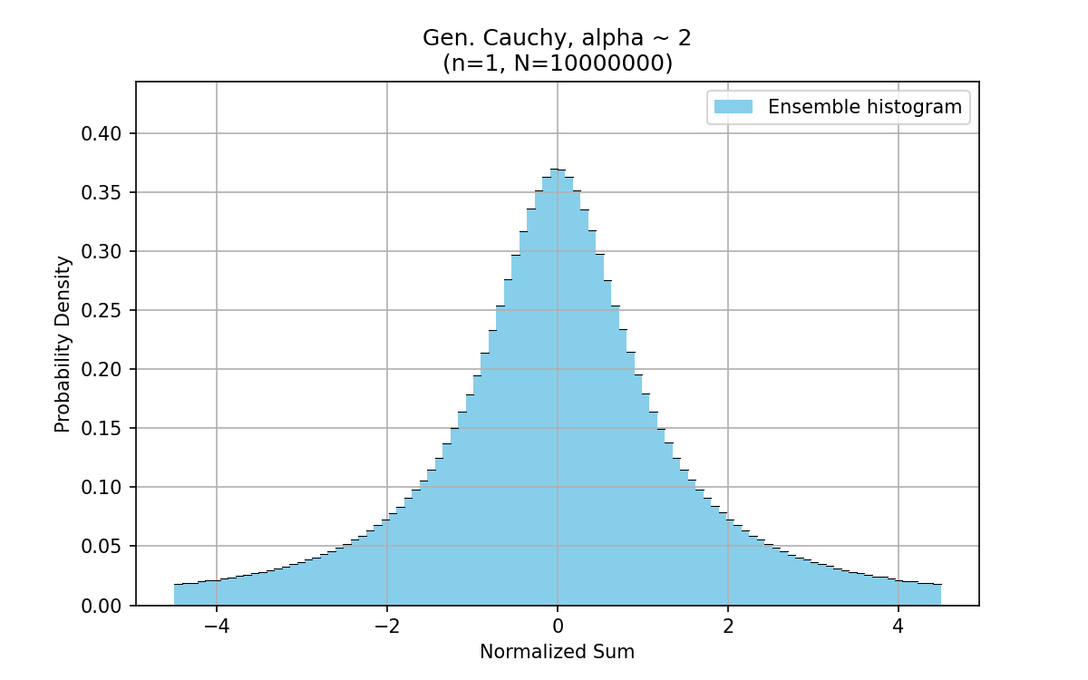
As we can see, the Cauchy distribution never truly strays from its original shape. With its very heavy tails ($f(x) \sim x^{-2}$), the Cauchy distribution lacks a well-defined mean or variance, and therefore doesn't satisfy the conditions of the central limit theorem. Nevertheless, for a carefully chosen width, its behavior under averaging can still stabilize in a meaningful way.
Why does the convergence towards a Gaussian happen analytically?
So far, we've explored the central limit theorem through numerical experiments - summing random values and watching the distribution approach a Gaussian. This analytical derivation complements our earlier Python demonstration, where we plotted the distribution of normalized averages for increasing $n$. Now, let's understand why the Gaussian appears so universally from a mathematical perspective. A powerful tool to approach such problem is the characteristic function.
What is a characteristic function?
For a random variable $x$, the characteristic function is defined as:
$$ \phi (t) = \left\langle e^{i t x} \right\rangle $$
This expression might be confusing, but it essentially means: given a random variable $x$, take the complex-valued expression $e^{i t x}$ where $t$ is some (real, for now) number and compute the average value of such expression. Since $t$ is in there, this will be a function of $t$ - the characteristic function! It captures the entire distribution and behaves nicely under addition of independent random variables, which is extremely useful for our purposes here.
AsideCharacteristic function of the Gaussian
Suppose $x \sim \mathcal{N}(0, 1)$, so the distribution of $x$ is $(2 \pi)^{-1/2} \exp ( - x^2 / 2)$. Its characteristic function is
We complete the square in the exponent:
So the integral becomes:
since the integral evaluates to 1 (just a shift of a normalized Gaussian). So:
This is the characteristic function of the standard normal distribution.
Step-by-step: what happens when we average?
Let's say $x$ is drawn from a distribution $\mathcal{D}(x)$ with mean zero and variance 1 (we can always shift and rescale to make this true). Now, define
$$ X = \frac{1}{\sqrt{n}} \left( x_1 + x_2 + \dots + x_n \right) $$
This is the average of $n$ independent samples, rescaled so that its variance stays equal to 1 no matter the value of $n$ (if you have a hard time believing that specifically factor $1/\sqrt{n}$ is needed to make this work, keep reading). We are interested in the characteristic function of $X$
$$ \phi_n (t) = \left\langle e^{i t X} \right\rangle $$
Since the $x_i$ are independent, this becomes:
where $\phi_1 (t)$ is the characteristic function of $x$.
Expanding the characteristic function
Let's expand the individual characteristic function $\phi_1(t)$ into a Taylor series. Assuming all moments exist, we get:
Where we used the fact that $\langle x \rangle = 0$ (zero mean) and $\langle x^2 \rangle = 1$ (unit variance). Recall we assumed this earlier for generality - any distribution with finite mean and variance can be rescaled to meet this. Now plug in $t/\sqrt{n}$ instead of $t$, and raise the whole thing to the power of $n$:
Watch the limit work
As $n \to \infty$, this product starts to resemble an exponential. To see that, recall this famous limit:
$$ \lim_{n \to \infty} \left( 1 + \frac{x}{n} \right)^n = e^x $$
Our expansion now becomes:
$$ \phi_{n \to \infty} (t) = \lim_{n \to \infty} \left( 1 - \frac{t^2}{2 n} + o (1/n) \right)^n = e^{-t^2 / 2} $$
And that is exactly the characteristic function of the standard Gaussian distribution. We can also see that the factor $1/\sqrt{n}$ was needed to exactly balance out the power of $n$, leaving a nicely behaving function behind.
This simple but powerful argument shows us why the Gaussian distribution emerges from summing up many independent contributions: the higher-order terms vanish in the limit, leaving only the second moment (the variance), which controls the width of the bell curve.
Beyond the limit: rate of convergence
We just showed why so many random additive processes converge to a Gaussian. We might, however, be interested in the rate of convergence towards this universal distribution. How high $n$ is high enough? For that we need to go back to the expression for $\phi_n (t)$ and its relation to $\phi_1 (t)$
$$ \begin{aligned} &\phi_n (t) = \left( \phi_1 (t / \sqrt{n}) \right)^n = \\ = &\left( 1 - \frac{t^2}{2n} - \frac{i \langle x^3 \rangle}{3! n^{3/2}} t^3 + \frac{\langle x^4 \rangle}{4! n^2} t^4 + \dots \right) \times \cdots \\ \times &\left( 1 - \frac{t^2}{2 n } - \frac{i \langle x^3 \rangle}{3! n^{3/2}} t^3 + \frac{\langle x^4 \rangle}{4! n^2} t^4 + \dots \right) \end{aligned} $$
To obtain the term-by-term expansion of this product, we'll start from the lowest power in $t$, building up. First, the only way we get a constant independent of $t$ is to take factor of $1$ from each bracket, which gives us again a factor of 1. The next lowest possible power in $t$ is $t^2$, which can be obtained by taking a term $t^2$ from one single bracket and $1$ from all others. Since there are $n$ total brackets, there will be $n$ such terms. This gives us the start of the expansion:
$$ \phi_n (t) = 1 - n\frac{t^2}{2 n} + \cdots = 1 - \frac{t^2}{2} + \cdots $$
As expected, we are starting to see the expansion for $\exp (- t^2 / 2)$ and $n$ has not appeared yet - the first two terms are independent of $n$. We can continue with the cubic term. Since none of the brackets contains a term linear in $t$, the only way to get a cubic term is to again take a single cubic term from one of the brackets and $1$ from all other brackets, resulting in
$$ \phi_n (t) = 1 - \frac{t^2}{2} - \frac{i \langle x^3 \rangle}{3! \sqrt{n}} t^3 + \cdots $$
We can see that in the limit $n \to \infty$, the cubic term vanishes, because it is proportional to $1/\sqrt{n}$. This is consistent with the limit being the characteristic function of the standard Gaussian, $\exp (- t^2 / 2)$, as it does not have skewness. The quartic term can be derived by collecting all the possible ways $t^4$ can occur in the result ($n(n-1) / 2$ ways to take the quadratic term from exactly 2 brackets + quartic term from a single bracket), we get
Here we see that when $n \to \infty$ the quartic term converges to $t^4 / 8$, which is the next expansion term for $\exp (- t^2 / 2)$.
We can see a very definitive result in these expansions: the rate of convergence toward a Gaussian depends on how quickly the higher-order terms vanish. If the original distribution has a nonzero skewness $\langle x^3 \rangle \neq 0$, the leading correction is of the order $1/\sqrt{n}$. If the skewness vanishes, the next correction (from $\langle x^4 \rangle - 3$) is of order $1/n$. If the distribution shares more moments with the Gaussian (zero odd moments, even moments $\langle x^{2k} \rangle = (2k-1)!!$), convergence can be even faster, though such cases occuring naturally are increasingly rare in practice.
This derivation reveals just how fundamental the Gaussian distribution is: averaging independent effects suppresses the contribution of all but the second moment, leaving behind the familiar bell curve. The speed at which this convergence occurs depends on the structure of the original distribution — symmetry and finite moments help the process along, but even asymmetric or jagged sources eventually yield.
But not all processes in nature are additive. Some involve multiplication, feedback, or nonlinearity, yet the Gaussian still shows up, sometimes where we least expect it. In part 3 we look at a few such examples and look for the Gaussian hiding under the hood.